Old Way (Serial)
New Way (Parallel)
By the early to mid 2000s, the physical limitations of semi-conductor based, microelectronics had begun to alter the course of processor design. Clock speeds, which had increased by several orders of magnitude in the latter part of the 20th century, could no longer be significantly enhanced. As a result, manufacturers began to focus more on parallel computing via multi-core processors in order to increase computing power. Since then, eight, 16 and even higher-core processors have since become more prominent in newer personal computers.
Beginning in the late 2000s, requests for PSCAD and EMTDC to take advantage of parallel computing techniques began to rise. In response to this increasing feedback, the development direction began to move in part towards the exploitation of multiple-core processors; this in order to increase simulation efficiency and reduce the time needed to extract results. Versions prior to v4.5 (released in 2012) did not utilize more than two processor cores. PSCAD and EMTDC ran on separate cores, but there was always only one EMTDC process running at any given time.
With the release of v4.5, two unique parallel computing functions were incorporated that both utilize multiple processor cores: A parallel solution of transmission lines and cables, and a rudimentary ability to launch multiple EMTDC simulation runs simultaneously, where each EMTDC runtime process is based on a unique case project. In v4.6, the ability to launch multiple EMTDC processes from a single project was introduced.
NOTE: A standard PSCAD license allows a maximum of eight simultaneous, parallel EMTDC simulations. For information on increasing this limit, contact the PSCAD Sales Desk (sales@pscad.com).
In older versions, transmission lines and cables were solved sequentially (i.e. one at a time). Some projects we have come across contain hundreds of transmission segments; the serial processing of which was cumbersome and time consuming. Given the fact that transmission lines and cables are solved independently of each other, and that there can be many of them in a single project, it makes perfect sense to exploit parallel computing techniques to solve them faster.
|
|
Old Way (Serial) |
New Way (Parallel) |
When a project is compiled, one of the final steps in the compilation process is to solve each and every transmission segment. Once this is complete, the EMTDC runtime executable can be built and the simulation launched. Transmission segments are now solved in parallel, based on the number of cores available on the local machine. For example, if the local processor has 8 cores, 7 of the 8 (one is being used by PSCAD) will be utilized until all segments are solved. Each segment will be assigned a single core directly: If the number of segments exceeds the number of cores available, then the segments will be solved in sequential sets until they all are solved. In the example above, note that only 7 segments are solved at a time, as there are only 7 cores available for processing.
Simulation sets are an inherent part of the workspace, and can be viewed and modified from within the workspace primary window.

The concept of a simulation set provides the foundation for parallel computing in PSCAD. A simulation set is a container of sorts, used to compartmentalize and configure groups of simulations. All simulations placed within a particular set are launched simultaneously (in parallel), utilizing all processing resources available. If multiple simulation sets have been defined, then each set is run sequentially as they appear in the list of sets: In the image above for example, SimulationSet1 will launch and run the ieee_ssr_bench and Study_2 projects simultaneously. Once finished, SimulationSet2 will launch and run the Cigre_Benchmark project. The sequential launching of all sets is automatic, if the user selects to run all sets.
The image below illustrates a scenario on how resources are utilized when running simulations in sets. In this example, there are two sets, one containing 5 simulations, and the other 9. As the local processor is 8-core, then there are 7 cores available (one used by PSCAD) to run the processes. The second set contains more simulations than there are cores available (9 simulations, 7 cores). In these situations, the operating system will force all 9 processes to be shared amongst the available resources, resulting in decreased efficiency. It is important to note then to avoid exceeding the resources available to you when launching sets. Obviously, the more cores available for parallel processing, the larger the sets of simulations can be without decreasing efficiency.
|
|
Set Containing 5 Simulations Uses One Core For Each Directly |
Set Containing 9 Simulations Must Share the 7 Cores Available (Decreased Efficiency) |
Only projects loaded under the Projects branch in the workspace primary window may be added as a Simulation in a Simulation Set. Simulation sets and corresponding settings are all stored as part of the workspace.
For more information on manipulating simulation sets, see the following topics:
Adding a Project to a Simulation Set
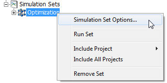
To invoke the Simulation Set Options dialog, right-click on an existing simulation set and select Simulation Set Options...
The following describes the options available for simulation sets:
Simulation Set
Name: The name of the simulation set. Name length must be 30 characters or less, and must only contain valid characters.
Command Line
Pre and post-run processes may be performed between simulation set runs. For example, a batch file can be used to copy or move EMTDC output files to another folder before the next simulation set is started.
Post-Run Process: Specify an executable (*.exe) or batch (*.bat) file to run, after the simulation set has completed.
Wait (Post-Run): Select Wait or Do Not Wait. If wait is selected, PSCAD will wait for the Post-Run Process to complete before continuing with the simulation set run.
Pre-Run Process: Specify an executable (*.exe) or batch (*.bat) file to run, before the simulation set has completed.
Wait (Pre-Run): Select Wait or Do Not Wait. If wait is selected, PSCAD will wait for the Pre-Run Process to complete before continuing with the simulation set run.
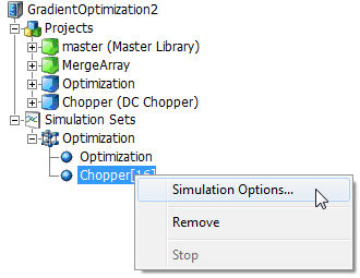
To invoke the Simulation Options dialog, right-click on an existing simulation and select Simulation Options...

The following describes the options available for simulations:
General
Namespace: Display only. This is the associated project namespace name.
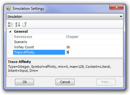
Volley Count: Each project can launch multiple instances of itself for batch processing, each assigned a rank number used to isolate control behaviour. See Volley Launch (SPMD) for more details.
Trace Affinity: Specify which project instance run (rank number) that will provide trace, or plotting information back to PSCAD. For example, if the Volley Count is set to 10, then there are 10 possible simulations that can be used as a 'tracer'. Select a single number (i.e. the rank number) to specify. See Volley Launch (SPMD) for more details.
In computing, the acronym SPMD (or 'spim-D') stands for Single Program, Multiple Data. It is a technique used to achieve parallelism, where multiple instances of a simulation are run simultaneously on multiple processor cores, given different input, in order to obtain results quicker and more efficiently than running them sequentially. In PSCAD, the SPMD concept is referred to more affectionately as a Volley Launch, analogous to the military tactic of having a line of soldiers fire all their weapons simultaneously. SPMD is also referred to as Data Parallel Processing.
Volley launch provides the ability to launch multiple simulation runs in parallel (up to a maximum of 64), based on a single case project. To set up a volley, a simulation must first be added to a simulation set. Once added, simply invoke the Simulation Options dialog and adjust the Volley Count option. For example, if you want to launch 7 simultaneous runs of a single project, then set the Volley Count to 7. When you next launch the simulation set, 7 instances of that simulation will be launched in parallel, utilizing all available processor cores.
In the example below, a project called Chopper is set to run as a volley of 16.
|
|
|
A Simulation Called Chopper Set to a Volley of 16 |
Simulation Options Dialog |
Volley Count Displayed on Simulation |
The Rank Number, or simply Rank, is an identification number for a single simulation instance that is part of a volley launch. If there are 16 simulation instances in a volley for example, rank number 5 identifies the 5th simulation instance.
When a simulation is launched as a volley, only a single simulation can be selected to pass plotting data back to PSCAD for display. The rank number is used to identify the simulation instance to be used as the tracer. Tracer is also a military term referring to tracer bullets used in automatic weapons — projectiles that are visible to the naked eye. The tracer simulation is set via the Simulation Options dialog, using the Trace Affinity field.
|
|
A Simulation Called Chopper Set to a Volley of 16 |
Simulation Options Dialog |
In the example above, the Trace Affinity is set to 3, meaning that the 3rd simulation instance in the volley will return the plotting waveforms. The purpose of this is to provide user feedback during development and debugging of the simulation. Once this part is complete, the affinity can be set to 0. Zero indicates that no simulation will return waveforms, resulting in better performance.
The rank number is also used to ensure unique input data for each simulation instance in the volley. Rank number can be used in combination with the Rank Number component in the master library.

The Root Control Interface (RCI) was first released as part of the v4.5 minor upgrade. Root control allows for one root, or master project, to control multiple slave projects, where both master and slaves must be part of the same Simulation Set. The idea behind the development of the RCI was to support both parameter sweep, as well as optimization-based, multiple-run studies.
Like the simulation sets, the RCI is an inherent part of the workspace, which enables inter-project communication within a single simulation set. This is accomplished using the already well defined Radio Link transmitter and receiver components, which were extended in v4.5 to include a provision field for a foreign namespace (that is, another project within the workspace). This instructs the link to collect its value from a foreign source, and thus allows for a more sophisticated means of multiple run control.
|
A Simulation Set with Three Projects: One Master and Two Slaves |
The image above illustrates an example simulation set containing three projects: One configured as a master and two configured as slaves. Each slave project communicates with the master via radio link transmitters and receivers. The master also communicates with the slaves in the same way. Communication between projects is performed only between runs; that is, following the end of one run and before the start of the next. In this way, the master project distributes the control parameters to the slaves, and the slaves send result data back to the master (via radio links). The master uses the results data from the slaves to generate input data before the next run starts.
To configure a project as master or slave, change the Run Configuration field under the Runtime tab in the project settings.
NOTE: Radio links possess an additional facility for the purpose of plotting its value for each run, within the master project.
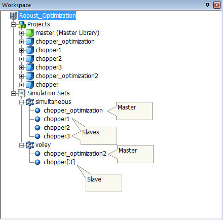
Consider the Robust Optimization example workspace in the PSCAD examples folder under ...\Examples\Root Control (start PSCAD and load this workspace if desired to better follow along with this example explanation). This workspace is composed of four projects, one configured as a master (chopper_optimization) and the other three as slaves.
|
The Robust Optimization Workspace |
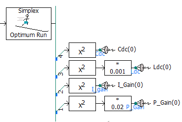
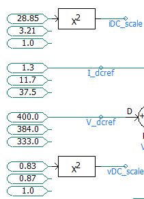
In this example, we focus on the simultaneous simulation set (non-volley), where three slave projects containing a chopper circuit are run in parallel for each multiple run. Before the start of each run, the master project (called chopper_optimization), which contains the Optimum Run component, provides each slave project with unique, initial data. The data provided to the slave projects is the DC parallel capacitor value Cdc, the DC series inductor value Ldc, and the proportional and integral gain values (I_gain and P_Gain) for the PI controller component. All four of these values are transmitted from the master to each slave project using radio links.
|
|
Data Transmitted from the Master Project |
Data Received by the Slave Projects |
NOTE: The rank number specified in each of the radio links is 0. This signifies that the signal is being transmitted to all simulation instances. In this example, there is only one simulation instance for each project.
Each chopper project is unique, in that the input constant tags in each control circuit are slightly different.
|
|
|
Project chopper1 |
Project chopper2 |
Project chopper3 |
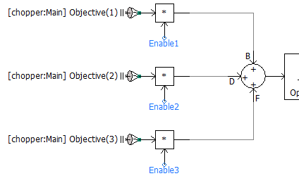
The differing inputs to the control circuit result in a unique output quantity from each slave. A single output signal, being the objective function (Objective) is transmitted back to the master via radio links.
|
|
Data Transmitted from the Slave Projects |
Data Received by the Master Project |
NOTE: The rank number specified in each of the radio links in the master is 1. This is because this is a non-volley simulation and so there is only one unique instance of each simulation.
The master project in this example contains a plot of the three, unique objective functions coming back from each slave case, where the x-axis is the multiple run number. See Running Simulations Sets for more.
|
Objective Function Trend Graph (Unique Objective Signal from Each Slave Project) |
Root control can also be used in combination with volley launch. Making use of volley launch will reduce the number of slave projects you need to maintain, down to just one. The volley rank number is then utilized to provide differentiation between simulation instances.
EXAMPLE B (Volley):
Consider again the Robust Optimization example workspace described above.
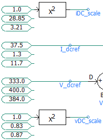
In this example, we focus on the volley simulation set, where a single slave project containing a chopper circuit is launched as a volley of three for each multiple run. As in EXAMPLE A, before the start of each run the master project (called chopper_optimization2), which contains the Optimum Run component, provides the slave project initial data. The data provided is the DC parallel capacitor value Cdc, the DC series inductor value Ldc, and the proportional and integral gain values (I_gain and P_Gain) for the PI controller component. All four of these values are transmitted from the master to the slave project using radio links.
|
|
Data Transmitted from the Master Project |
Data Received by the Slave Project |
NOTE: The rank number specified in each of the radio links is 0. This signifies that the same signal is being transmitted to all simulation instances in the volley. In this case, all three simulation instances will receive the same data values from the master.
The chopper slave project is being launched as a volley and so all simulation instances will be identical. As such, we must rely on the simulation rank number in order to provide each simulation instance with unique values. The input constant tags that were made unique in each slave project in EXAMPLE A, have been moved to the master project in this example, and then the data transmitted to each simulation instance via the rank number.
|
|
Data Transmitted from the Master Project |
Data Received by the Slave Project |
NOTE: A unique set of three values needed by each simulation instance are transmitted from the master, given a specific rank number. A rank number of 0 is specified in the slave to indicate that it should only receive transmitted data matching it's rank number.
A single output signal, being the objective function (Objective) is transmitted back to the master via a radio link.
|
|
Data Transmitted from the Slave Projects |
Data Received by the Master Project |
NOTE: The rank number is specified in each of the radio links in the master.