Cut/Copy/Paste an Existing Curve
Synchronizing Output Channel Limits with Those of the Graph
Curves Sourced from Multiple Instance Modules
A curve is special runtime object best described as a graphical representation of a string of data points, where each point is associated with a simulation plot step. Curves are created by linking to an Output Channel component, to which a scalar or array set of data signals have been input. As such, curves can be multi-dimensional; that is a single curve may possess many sub-curves or Traces, where each trace corresponds to a single array value.
If the Output Channel input signal is a scalar (i.e. single dimension), then the curve will consist of a single trace. For more information on accessing and adjusting individual trace properties, see Traces.
Adding a curve to a graph can be accomplished a couple of different ways:
Drag and Drop Method: Hold down the Ctrl key. Left-click and hold over the output channel component from which you would like to extract the curve. Drag the mouse pointer over a graph and release the mouse button. See Drag and Drop for more details on this.
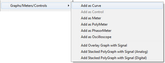
Graphs/Meters/Controls Method: Right-click on the output channel component from which you would like to extract the curve. Select Graphs/Meters/Controls | Add as Curve. Select the desired graph with a left-click, then right-click and select Paste Curve.
Once a curve has been added to a graph, the curve title will appear in the curve legend.
Once multiple curves have been added to a graph, you may change the order in which they appear. Ordering curves can be accomplished in one of two ways:
Drag and Drop: Left-click and hold over the curve in the curve legend. Drag the mouse pointer to a new position in the curve legend and release the mouse button. See Drag and Drop for more details on this.
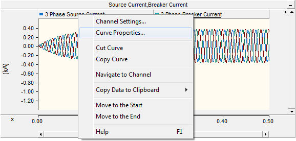
Right-Click Menu: Right-click over the corresponding curve legend and select one of the following from the pop-up menu: Move to the Start or Move to the End.
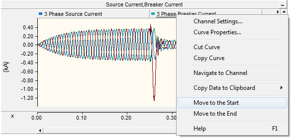
Right-click over the curve title and select either Cut Curve or Copy Curve, depending on what you want to do. Right-click over any graph and then select Paste Curve to paste the curve. The curve should then appear in the corresponding curve legend.
If a simulation has been run and a particular curve contains data, you have the option of copying all or a portion of this single curve data set to the clipboard. Right-click over the corresponding curve name, select Copy Data to Clipboard and then select one of the following from the pop-up menu:
All: Copies all curve data available
Visible Data: Copies only curve data that is visible in the graph window.
Between Markers: Copies only curve data situated between markers. Note that Show Markers must be selected in the Axis Properties dialog.
The data is copied as Comma Separated Variables (*.csv) format for easy migration into common data analysis software.
Left double-click on the desired curve in the curve legend, or right-click the curve and select Curve Properties....
This will bring up the Curve Properties dialog window.
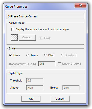
The following list describes the parameters in this section:
Display the active trace with a custom style: Select this option if you wish to change the colour or width of the active trace.
Colour: Press the Colour... button to select a display colour for the trace. Press the OK button in the colour dialog. This option is enabled only if Display the active trace with a custom style is selected.
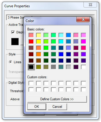
Bold: Select this option if you wish the trace to appear bold. This option is enabled only if Display active trace with a custom style is selected.
The following list describes the parameters in this section:
Lines: Displays the curve as a standard line.
Points: Displays the curve as a series of points according to the set plot step.
Filled: Fills the area under the curve (between the curve and the 0.0 line) with the curve colour.
Transparency (1-255): Sets the transparency level of the filled portion under a curve. This is adjustable only when Filled is enabled.
Linear Gradient: Select this option to create a linear gradient effect on the filled part under the curve. This is adjustable only when Filled is enabled.
These options are only considered if the curve is part of a polygraph. Digital style controls the properties the curve traces when they are in digital mode. The following list describes the parameters in this section:
Threshold: The threshold value at which to change the display state of the curve.
Above / Below: Enter the state for the curve when value is above and below the set threshold respectively.
The source Output Channel parameters for a particular curve can be accessed directly from the curve legend pop-up menu. Right-click the curve and select Channel Settings....
Once one or more curves have been added to an overlay graph, all corresponding Output Channel component Min / Max limits can be synchronized to the graph y-axis minimum and maximum limits.
To synchronize output channel limits with the graph, right-click over the overlay graph and select Synchronize Channel Limits to Graph.
Module components can possess more than one instance. This means that if an Output Channel exists on the canvas of a module (i.e. part of the module definition), then it will produce a unique curve for each instance of the module, even though there is technically only a single Output Channel component. If the curve associated with the Output Channel is placed in a graph that exists outside the module, which unique curve instance is displayed?
Each curve instance is referred to as a call. If a curve exists in a graph that is sourced from an output channel inside a multiple instance module, then you can access and control the view of any number of the unique calls. Simply hold down the Ctrl key and left-click on the curve legend. A display list will appear showing all source curves (calls) available.
In the above image, it is apparent that the curve Data is sourced from 16 different module instances that are based on the same definition. In this particular example, call 0 (base 0) and call 4, 6 and 15 are being displayed. You may choose to display all calls in a single graph, or you can place the Data curve in multiple graphs, and select a unique call to display in each graph.
For more information on multiple instance modules, see Multiple Instance Modules (MIM).