The Bergeron Model

Bergeron Method vs. Multiple P-Sections

Inclusion of Line Resistance

Time Domain Implementation

Frequency for Loss Approximation

The Bergeron model is closely related to the Method of Characteristics described in the previous section.  That is, it is essentially an ideal (loss-less) model represented by a distributed inductance L and a capacitance C.  However, the Bergeron model goes a step further to include a lumped resistance property to approximate system losses [6].

It is important to note that the Bergeron model is a single-frequency model.  That is, all calculated parameters, such as characteristic impedance Z0, are calculated at a specified frequency:  Usually either 50 or 60 Hz for an AC transmission line.  Although the Bergeron model can indeed be used for transients simulation in the time domain (which includes all frequencies), only results at the specified steady-state frequency are meaningful.  As such, the Bergeron model should only be used for general fundamental frequency impedance studies, such as relay testing or matching load-flow results.

Bergeron Method vs. Multiple P-Sections

The Bergeron model should generally be chosen over a p-section equivalent whenever the system length is sufficient enough to allow the propagation of waves (at approximately the speed of light) to travel the entire length of the line within a single time step.  This means that for a typical simulation time step of Dt = 50 ms, transmission systems roughly over 15 km in length should be represented by the Bergeron model as opposed to a p-section.  The advantages are of course that a real world propagation delay is considered in the Bergeron model, and also that series connected p-sections can introduce artificial resonances at high frequencies [6].

Inclusion of Line Resistance

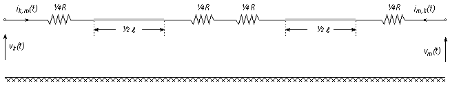
The Bergeron model approximates losses by adding series lumped resistance elements into the loss-less, distributed parameter branch defined by the Method of Characteristics.  Given the total system resistance R (as calculated by the PSCAD Line Constants Program), the loss-less line is broken into two segments, each with a ¼R resistance at each end.  When these segments are combined, a lumped resistance of ½R in the middle and ¼R at each end results [6, 19].

Figure 8-33 – Loss-Less Line with Lumped Resistance Included

Where,

The breaking of the system into two sections, along with the additional resistance elements, results in a change in the Norton representation of the loss-less line shown in Figure 8-33.  The equivalent circuit of a loss-less line with lumped line resistance is given below:

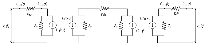
Figure 8-34 – Loss-Less Line with Lumped Resistance Equivalent Circuit

Time Domain Implementation

The circuit of Figure 8-34 can be collapsed into the same two-port format as the Distributed Branch Interface in Figure 8-32 (shown again below):

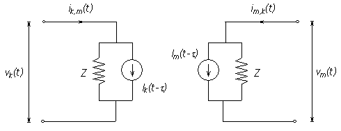
Figure 8-35 – EMTDC Bergeron Model Time Domain Interface (Single-Phase)

The Norton interface impedance Z at each end of the line now becomes:

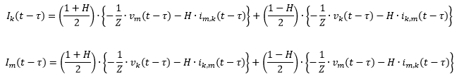
The change in Norton impedance Z is reflected in the definition of the Norton current injections Ik and Im as follows:

Where,

Frequency for Loss Approximation

The Bergeron model can actually calculate at two frequency points:  The second point being a frequency chosen by the user (greater than the fundamental), for the specific purpose of providing additional attenuation at high frequencies.  Note that the transmission system is not modeled exactly at the higher frequency because the characteristic impedance, travel time, etc., are still those calculated at the fundamental frequency.

NOTE:  This option can be invoked by choosing the 'Use Damping Approximation?' option in the Bergeron model.

Upon assembly of the of the Bergeron model interface, EMTDC will create a split at the log average wm of the two specified frequencies and determine the high and low frequency attenuation paths:

Where,

The frequency for loss approximation w1 is normally selected to be in the range between 100 Hz and 2 kHz, which may be chosen to accommodate specific resonance conditions of interest.

The log average frequency wm is used to calculate the real pole time constant tc = Dt.wm, which is applied to the Bergeron model interface.

Shaping Time Constant

If a high frequency loss approximation is indeed performed, then the current is processed through a real pole with a shaping time constant of tS just before being injected into the line terminations.

Selection of the wave shaping constant tS can be made in order to shape the steep front of a travelling wave to a known attenuation and slope.  If one is concerned about matching the steep front from the Bergeron line model to a known response, tS must be adjusted by trial and error.  Care should be taken when using the wave shaping time constant, because although the real pole will attenuate the high frequency components of the line, it will also introduce an additional lag or time delay, which in turn affects the overall travel time and thus, the effective line impedance.

EXAMPLE 9-1:

Consider a single-phase Bergeron line model connected to an infinite source and terminated with a large resistance.  

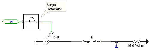
Figure 8-36: Single-Phase Bergeron Transmission Line in PSCAD

A voltage surge is applied at the sending end of the line, and the resultant sending end current is monitored.  The waveform is compared to the sending end current given by the Frequency Dependent (Phase) model, which for this example is assumed to very similar to a real world result.

NOTE:  This option can be invoked by choosing the 'Use Damping Approximation?' option in the Bergeron model.

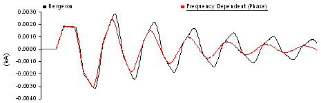
Figure 8-37 – Bergeron Response without High Frequency Attenuation

Due to the lack of high frequency attenuation in the Bergeron model, the receiving end voltage includes frequency components of higher order (as witnessed by the extra 'sharpness' of the reflections).

If the 'Use Damping Approximation' is enabled in the Bergeron model, then a more accurately attenuated current is produced.  However, note that a phase shift has been introduced by the wave shaping real pole function.

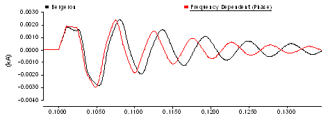
Figure 8-38: Bergeron Response with High Frequency Attenuation

For this example, the parameters were as follows: