Equivalent Conductance (GEQ) Electric Interface

General Considerations

Custom Current Source and Conductance Interface

Runtime Configurable Passive Branch

Control of the GEQ Interface from PSCAD

The equivalent conductance (or GEQ) interface provides the user with a straightforward method of interfacing electric models to the greater electric network.  Introduced with the release of EMTDC V3, the GEQ interface is an enhancement to the now obsolete, nodal-based GDC and GDCS interfaces used in EMTDC V2.  It is also an enhanced alternative to the node-to-node GGIN interface, which is deprecated and will slowly phased out over time.

These older interfaces were hindered by the fact that their parameters were indexed by way of node number, rather than by branch.  Problems with these interfaces arose when connecting several of them in parallel.  Due to the fact that each parameter was indexed according to node, each paralleled branch would have the exact same index, and so additional steps by the user were required to merge the branches into a single equivalent branch.  Also, extracting branch specific quantities, such as branch current was a bit convoluted.

The GEQ interface is virtually identical to the obsolete GDC interface, except that the parameter names and indexing have changed – one of its nodes can be grounded if desired as well.  Each parameter is indexed by a branch number directly, thereby enabling the extraction of branch data more easily.  The GEQ interface is illustrated below, where BRN represents the branch number and SS is the subsystem number:

Figure 5-3 – Equivalent Conductance (GEQ) Interface Branch

k and m are referred to as the ‘from’ and ‘to’ nodes respectively.   The parameters shown in Figure 5-3 represent the electrical functions of the GEQ interface, where EBR is an internal, ideal voltage source; GEQ and CCBR are the Dommel equivalent conductance and history current respectively, and CBR contains the calculated branch current.  These parameters are described in more detail later on in this section.

One advantage to using the GEQ interface over say, CCIN and GGIN (described later on), is that the branch history current (CCBR) is calculated by EMTDC automatically for LC branches.  Also, the user need only provide the conductance (and other branch information) once at the beginning of the simulation (unless of course the branch is a switching branch).

The GEQ interface can be set-up to represent any combination of series RLC passive elements, and along with its internal voltage source, can represent network equivalents.   It is also possible to set-up and control the GEQ interface to model non-linear impedances.

General Considerations

The GEQ interface is primarily used to represent branches consisting of series-connected R, L and/or C elements.  Any series combination of such elements is reduced by EMTDC into a single lumped admittance, represented by a Dommel equivalent, Norton conductance and current source (GEQ and CCBR).  The design process is somewhat automated where instead of relying on the user to directly calculate quantities each time step, the approach here is to provide EMTDC with information on how the branch is constructed, and what it consists of.  This information is given once at the beginning of the simulation (or whenever an R, L or C value changes), and then EMTDC handles the rest, such as internal node voltages and branch history currents.

The GEQ interface relies on the settings of certain parameters in order to effectively reduce a combination of elements to its Dommel equivalent.  This reduction is accomplished in two stages:  First, each element is reduced to its respective Dommel equivalent, and second, these individual circuits are merged into a single, lumped equivalent.  

Figure 5-4 – Steps in the Reduction of an RLC Branch Impedance to a Lumped Dommel Equivalent Circuit

Although the process for deriving the reduced branch conductance is relatively straightforward, deriving the equivalent history current IH is not.  The history current derivation depends on combinations of ratios between individual conductance values in the branch, which can be quite elaborate.  Nonetheless, users must supply this information to EMTDC and fortunately, the GEQ interface provides an avenue to do this easily.

Custom Current Source and Conductance Interface

A simple interface routine is provided so that users do not have to set global variables related to the branch manually. To use the current source and conductance interface, the user must add the following script to the Branch segment of the user component definition.

Listing 5-11 – Example Branch Section Script for a Custom Current Source and Conductance Branch

BR is the symbolic branch name, $A and $B are the end nodes of the branch. The default resistance of the branch is set to 1.0 .

Once a branch has been designated as shown above, the user must enter specific subroutine calls within the component definition DSDYN or Fortran segments (or directly within the user-written subroutine for the model). Within #BEGIN/#ENDBEGIN directives, there should be a call to the CURRENT_SOURCE2_CFG routine.

Listing 5-12 – Example Code for a Custom Current Source and Conductance Branch (Configuration)

Where $BR and $SS are the predefined branch number and subsystem number respectively.  This subroutine sets the internal EMTDC variable DEFRDBR($BR,$SS) to .TRUE., which is required to enable the custom current interface using the CCBR($BR,$SS) branch history current.  If a call to CURRENT_SOURCE2_CFG is not provided, the CCBR variable for this particular branch is ignored.  CURRENT_SOURCE2_CFG also sets the branch conductance GEQ($BR,$SS) to zero, and removes this branch from being used by the harmonic impedance solution.

In the main body of the DSDYN or Fortran segments, users must set the branch GEQ and CCBR by calling CURRENT_SOURCE2_EXE routine.

Listing 5-13 – Example Code for a Custom Current Source and Conductance Branch (Executable)

Where COND is the actual conductance value and CUR is the injected current value.  If the conductance value changes at every time step, then it is advisable to ensure that nodes A and B, as defined in the component Branch segment above, are switched node types.

Runtime Configurable Passive Branch

If the requirement is a simple passive branch, where the RLC values need be assigned in the BEGIN section at TIMEZERO, then the following method can be used.  Define a passive branch in the Branch segment and then modify the branch variables in the DSDYN segment within #BEGIN/#ENDBEGIN directive.

Listing 5-14 – Example Branch Section Script for a Runtime Configurable Passive Branch

BR is a symbolic branch name, $A and $B are the end nodes of the branch. The default resistance is 1.0 , inductance 0.1 H and capacitance 1.0 F.

Once a branch has been designated as shown above, the user must enter specific subroutine calls within the component definition DSDYN segment (or directly within the user-written subroutine for the model). Within #BEGIN/#ENDBEGIN directives, there should be a call to E_BRANCH_CFG routine.

Listing 5-15 – Example Code for a Runtime Configurable Passive Branch (Configuration)

Where,

Table 5-7 – Argument List for the E_BRANCH_CFG Routine

Care should be taken not to pass a zero or negative value to any of the R, L or C arguments. There should be conditional logic to set the values of ER, EL and EC depending on the values of R, L and C.  If ER is enabled and R value is less than the ideal threshold, then the resistive portion of the branch would be modeled as a short.  If ER, EL and EC are all disabled, then the branch is modeled as an ideal open circuit.

Control of the GEQ Interface from PSCAD

Everything discussed thus far regarding the GEQ interface can accomplished directly within the component definition, without the need for calls to external code.  That is, it is not necessary for the user to define the GEQ interface parameters through code, if designing a simple RLC branch with or without an internal source.

There are two avenues through which the GEQ interface can be controlled, these are:

1. The Branch segment in the component definition Script section

2. Utilizing the E_VARRLC1x internal subroutines.

The Branch segment is normally selected if the user wishes to create a simple, static RLC branch (with or without an internal source).  The E_VARRLC1x subroutines can be used for this purpose as well, but with the added ability for the online control of a single, non-linear R, L or C element in a branch.

Branch Segment

The Branch segment in the component definition Script section can be used to directly define one or more GEQ interface branches.  Here, the user simply needs to create a new component, and enter the R, L and/or C values directly into a defined branch.  EMTDC will automatically set-up the required flags, parameters and ratios for you.

EXAMPLE 5-3:

A user wants to create a new component, which will represent a 3-phase, Y-connected RLC constant impedance with R = 1.2 , L = 0.053 H and C = 33.3 F.  A new component is created with 4 electrical connections named NA, NB, NC (phase nodes) and GND (common node).

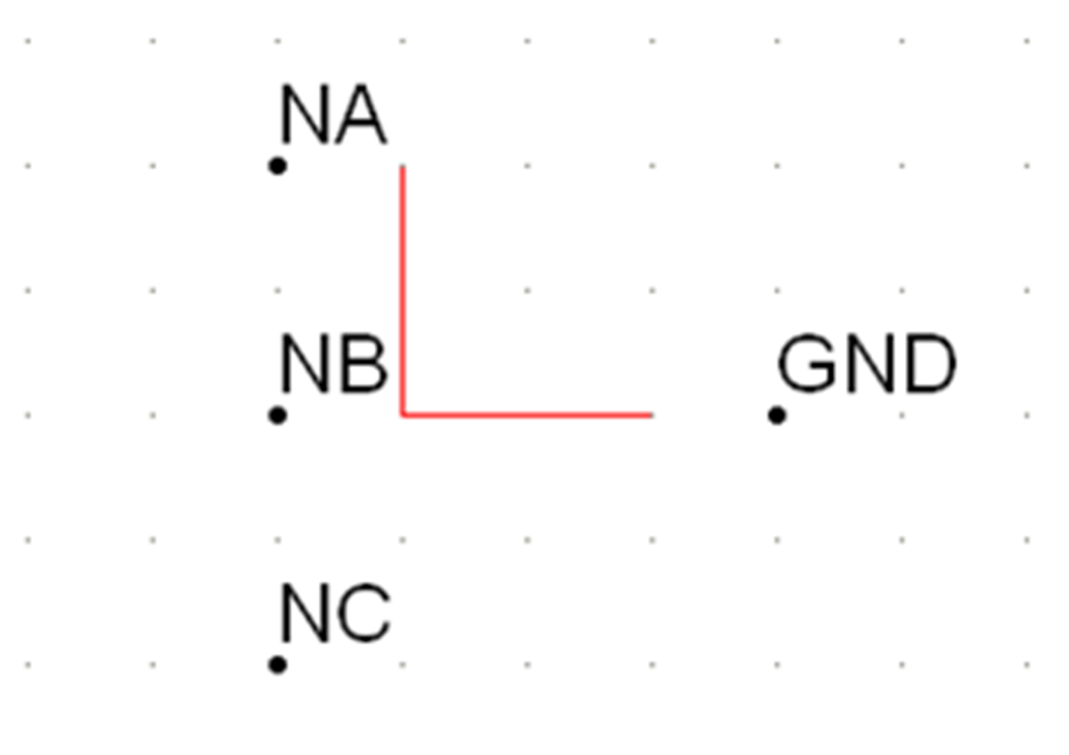
Figure 5-5 – Electrical Port Connections Defined in the Graphics Section of the Component Definition

A Branch segment is added and the three, Y-connected branches are defined as shown below as it would appear in the Branch segment:

Listing 5-16 – Example Branch Section Script for a Static RLC Branch

The above script will define three separate, series RLC branches, which use the GEQ interface.  See the section entitled Segment Types in the chapter Component Design of the PSCAD Manual for more details on defining branches.

If the user wishes to enable and control the internal branch voltage source EBR, then a slight modification is required to Example 5-3:

EXAMPLE 5-4:

A user wants to create the exact same 3-phase, Y-connected load as described in Example 5-3.  However an internal branch voltage is also to be included.  The component still consists of four electrical connections, but the Branch segment must be modified as shown below:

Listing 5-17 – Example Branch Section Script for a Static RLC Branch with Internal Voltage Source

The additional SOURCE script in each branch effectively enables the EBR internal branch source in the GEQ interface.  EMTDC will then expect a value for EBR to be defined by the user each time step.

E_VARRLC1x Subroutines

These subroutines are included within EMTDC and may be called directly from the Fortran, DSDYN or DSOUT segments of any user defined component definition.  They allow the user to directly model either a linear or a non-linear R, L or C passive element, as well as provide control of the internal source, EBR.  Although this subroutine is, for the most part, a direct link to the GEQ interface, it is limited to the fact that only a single R, L or C element can exist in a single branch.

The subroutine call statements and argument descriptions are given as follows:

      CALL E_VARRLC1_CFG(RLC,M,NBR,NBRC)

      CALL E_VARRLC1_EXE(RLC,M,NBR,NBRC,Z,E)

Where,

Table 5-8 – Argument Descriptions for the E_VARRLC1_CFG and E_VARRLC1_EXE Subroutines

Note that the E_VARRLC1x subroutines are optimized for the control of non-linear passive elements.  It should not be used to represent constant elements, as the branch cannot be collapsed with other series elements in the circuit.  This can result in additional nodes, and slower simulation times.  See the section entitled Equivalent Branch Reduction in the chapter entitled Electric Network Solution for more details on this.

EXAMPLE 5-5:

In this example, the E_VARRLC1x subroutines are called from the Fortran segment of a user defined component definition, with its various arguments pre-defined as needed.   The Fortran segment of the user component is shown below:

Listing 5-18 – Calling the E_VARRLC1x Subroutines within the Component Definition

Here, both the E_VARRLC1_CFG and E_VARRLC1_EXE subroutines are configured to model a non-linear inductor (i.e. input argument 1), where the inductance is controlled by the input argument L.  E controls the internal voltage source EBR.  BRN and SS are the branch number and subsystem number respectively.

The branch number is defined in the Branch segment of the component definition as follows, where NA and GND are electrical nodes:

Listing 5-19 – Branch Segment Script to Coincide with E_VARRLC1x Subroutine Calls