The system dynamics is an essential part of the EMTDC solution process. It serves to encompass the electric network, providing the ability to interface with it on either side: Data may be controlled from one side, while extracted from the other.
Essentially a Fortran program in its own right, the system dynamics is built according to customizable specifications. These specifications are normally provided through PSCAD, in the form of components and modules. Components and modules are graphical representations of how the final program is to be structured, where each module, including the main page, is represented by a unique Fortran file. This file consists of declarations for a DSDYN subroutine, a DSOUT subroutine, and two BEGIN subroutines. Components always exist within modules, so as such they represent inline code that combines to define the contents of each subroutine.
Of course, some components are electrical in nature and hence provide information for the construction of the electric network as well. This information is collected and inserted into a Data file, where each module in a project possesses its own unique Data file. Data files are discussed in more detail later on in the section entitled Electric Network Solution.
The DSDYN and DSOUT subroutines provide accessibility for control and monitoring of system variables on either side of the electric network. This offers a great advantage in programming flexibility, as it enables both the control of input variables and the monitoring of output variables, all within the same time step. This is an important concept, especially in the design of control systems involving feedback: Judicial selection of code placement can help avoid time delays that are uncharacteristic to the real system being modeled.
When it pertains to source code insertion into the system dynamics, there is no difference between DSDYN and DSOUT, besides their sequence in the solution process. However, there are specific uses for each, and certain code may be more optimally utilized when it is placed in one, rather than the other. For example, DSOUT is primarily used to define output variables directly following the electric network solution. Of course, DSDYN could be used for this purpose as well, but the same output variables would be delayed, due to the time step increment between DSOUT and DSDYN (see Figure 2-1). Likewise, variables controlling electric devices (i.e. network input variables) are best defined in DSDYN, as then updates will occur in the same time step before the network solution.
Component source is inserted in either DSDYN or DSOUT, depending on what the component is connected to. Decisions are made by an involved internal algorithm in PSCAD, which ensures that both feedback and feed-forward signals are properly sequenced, minimizing time delays. However, component source may also be forced into either DSDYN or DSOUT at the user’s discretion. To force source script into a specific subroutine, use either the DSDYN or DSOUT script segments. To utilize the internal algorithm, use the Fortran script segment. For more details on these segments, see the section called Segment Types in the Component Design chapter of the PSCAD Manual.
As mentioned above, it is important to establish the proper use of DSDYN and DSOUT to avoid unnecessary time step delays. Meters used for the measurement of voltage and currents for example, are primarily defined in DSOUT: This is the logical subroutine to choose, as DSOUT will supply the measured quantities directly following the network solution. However, measured quantities are often used as inputs to control systems, where the individual control components are defined in DSDYN. Since there is a time step increment between DSOUT and DSDYN, the control system may be basing outputs on quantities defined in the previous time step.
EXAMPLE 2-1:
Figure 2-3 - Simple Comparator Circuit created in PSCAD
Consider the simple circuit in Figure 2-3. A comparator is being used to compare a real constant variable equal to 0.0, with a data signal Ea, which is a measured voltage from a voltmeter. The comparator is adjusted so as to give a high output when Ea becomes greater than 0.0, and a low output otherwise. The comparator dynamics are defined by default in the DSDYN subroutine, whereas the measured voltage signal Ea is defined in DSOUT as an output quantity.
With the above configuration, the comparator output signal will contain a single time step delay. This is due to the fact that the comparator dynamics in DSDYN (i.e. the code that determines its output state) are using a measured voltage Ea, defined in DSOUT. Since the comparator output state is based on the comparator inputs, the output will appear to have been delayed by one time step.
This delay can be removed simply by forcing the comparator dynamics code from DSDYN to DSOUT. This will force the comparator to consider the measured voltage within the same time step, when determining its state.
The BEGIN subroutine is used for time zero operations, such as variable initialization and storage. Although the use of BEGIN is not mandatory, it is required if a component is to support its use within modules with multiple instances. Components with source specified for the BEGIN subroutine are said to be Runtime Configurable.
The primary purpose of BEGIN source is to ensure that variables required for a particular component instance, are initialized and stored for use later during runtime. All components with BEGIN subroutine source will have their variables stored in sequence (according to where the component source appears in the system dynamics), to be later accessed in the same sequence during the main runtime loop. Component parameter values are thereby unique for each instance. This enables components that are defined as part of a module definition, to retain different parameter values in different instances of that module.
For example, Listing 2-1 illustrates snippets of code taken from a module Fortran file. The module contains an instance of the PI Controller component from the master library. Notice that in the BEGIN section, data is stored (in this case the initial output value), and then extracted again in the same sequence during runtime in the DSDYN subroutine.
|
! 90:[pi_ctlr] PI Controller RTCF(NRTCF) = 1.57 NRTCF = NRTCF + 1 |
|
! 90:[pi_ctlr] PI Controller RVD1_1 = RTCF(NRTCF) NRTCF = NRTCF + 1 |
|
|
|
|
|
BEGIN Subroutine |
|
DSDYN Subroutine |
Listing 2-1 - Variables Stored Sequentially in BEGIN and then Extracted During Runtime
See EMTDC Storage Arrays in the chapter entitled Custom Model Design for more details.
As mentioned above, a module definition is equivalent to a subroutine declaration in the system dynamics structure; where an instance of said module is analogous to a subroutine call. Considering that the system dynamics is partitioned into three separate sections (i.e. DSDYN, DSOUT and BEGIN), where BEGIN is further subdivided into two parts, module representation is not accomplished by a single subroutine, but a group of four – one to represent each dynamics section and subsection. All four subroutines are organized into a single Fortran file, where this file (along with a Data file) forms the definition of the module, in the same way as a definition is the foundation of a regular component.
Components existing within a module are combined to define the subroutine body, by insertion of their script inline, according to their sequence and placement on the module canvas: The actual source code is extracted from components, derived from definition script that exists in either the DSDYN, DSOUT or Fortran segments. Figure 2-4 and Listing 2-2 combine to illustrate this concept.
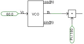
Figure 2-4 – Example Module Circuit Canvas
|
! SUBROUTINE DSDyn() ! ! . . . ! ! 10:[const] Real Constant RT_2 = 60.0 ! 20:[vco] Voltage-Controlled Oscillator ! Voltage Controlled Oscillator RT_1 = STORF(NSTORF) IF(RT_1.GE. TWO_PI) RT_1 = RT_1 - TWO_PI IF(RT_1.LE.-TWO_PI) RT_1 = RT_1 + TWO_PI RT_4 = SIN(RT_1) RT_3 = COS(RT_1) STORF(NSTORF) = RT_1 + DELT*RT_2*TWO_PI RT_1 = RT_1*BY180_PI NSTORF = NSTORF + 1 ! 30:[emtconst] Commonly Used Constants (pi...) RT_6 = PI_BY180 ! 40:[mult] Multiplier RT_5 = RT_1 * RT_6 ! ! . . . ! RETURN END
|
Listing 2-2 – Snippet of Inline Code from Module Fortran File (DSDYN Subroutine)
Figure 2-5 and Listing 2-3 illustrate how system dynamics files would be prepared upon building an example project. The project shown consists of the default Main module, which harbours two instances of a module called Module_1 along with a single instance of a component called Comp_1. Module_1 itself contains a single component instance called Comp_2.
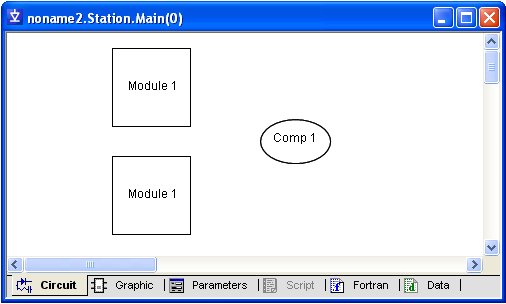
Figure 2-5 – Example Main Module Circuit Canvas
|
! SUBROUTINE DSDyn() ! ! . . . ! ! 10:[Module_1] CALL Module_1Dyn() ! 20:[Module_1] CALL Module_1Dyn() ! 30:[Comp_1] ... ! ! . . . ! RETURN END ! SUBROUTINE DSOut() ! ! . . . ! ! 10:[Module_1] CALL Module_1Out() ! 20:[Module_1] CALL Module_1Out() ! 30:[Comp_1] ... ! ! . . . ! RETURN END ! SUBROUTINE DSDyn_Begin() ! ! . . . ! ! 10:[Module_1] CALL Module_1Dyn_Begin() ! 20:[Module_1] CALL Module_1Dyn_Begin() ! 30:[Comp_1] ... ! ! . . . ! RETURN END ! SUBROUTINE DSOut_Begin() ! ! . . . ! ! 10:[Module_1] CALL Module_1Out_Begin() ! 20:[Module_1] CALL Module_1Out_Begin() ! 30:[Comp_1] ... ! ! . . . ! RETURN END
|
|
! SUBROUTINE Module_1Dyn() ! ! . . . ! ! 10:[Comp_2] ... ! ! . . . ! RETURN END ! SUBROUTINE Module_1Out() ! ! . . . ! ! 10:[Comp_2] ... ! ! . . . ! RETURN END ! SUBROUTINE Module_1Dyn_Begin() ! ! . . . ! ! 10:[Comp_2] ... ! ! . . . ! RETURN END ! SUBROUTINE Module_1Out_Begin() ! ! . . . ! ! 10:[Comp_2] ... ! ! . . . ! RETURN END |
|
|
|
|
|
Main.f |
|
Module_1.f |
Listing 2-3 – Assembly of System Dynamics Subroutines
Following a build operation, this project will possess two Fortran files: The first represents the definition of the Main module (Main.f), and the second the definition of Module_1 (along with their corresponding Data files). Each file contains four, separate subroutines corresponding to the three system dynamics sections. The subroutine names are pre-pended by the name of the module.
Note that although there are two instances of Module_1, they are both based on the same definition (i.e. Fortran file). Modules with multiple instances can still be unique however, through the use of its argument list. Subroutine arguments are used to pass both port connections and module input parameter values.
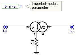
Consider a user-defined module, which represents a 3-phase, 2-winding Y-D transformer. The module canvas consists simply of a 3 Phase 2 Winding Transformer component from the master library, set as Y-D, with a 1 W resistance connected to the common of the primary winding. It is required that this components 3 Phase Transformer MVA input parameter be changeable on a per-module instance basis.
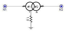
Figure 2-6 – Simple 3-Phase, 2-Winding Transformer Module Canvas
If this module is to be multiply instanced, then all components forming the module must be Runtime Configurable. Fortunately, the transformer component used in this module is such. To be runtime configurable means that components will make use of the BEGIN section of the system dynamics if required. However, only those component input parameters defined as Constant or Variable may be adjusted on a per-module instance basis (Literal parameters cannot).
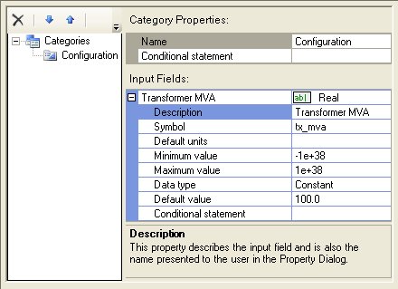
The 3 Phase Transformer MVA input parameter in the 3 Phase 2 Winding Transformer component is fortunately defined as a Constant. Therefore, in order to allow adjustment of this parameter on a per-module instance basis, an input parameter will need to be defined for the module itself, and the parameter value imported onto the canvas. A Constant type module parameter with Symbol name tx_mva is created and given a value of 100.0 MVA. Its corresponding Import tag is added to the canvas. The value of the 3 Phase Transformer MVA input parameter in the 3 Phase 2 Winding Transformer component is also entered as tx_mva.
|
|
|
|
|
|
|
|
|
Module Definition Parameters Section |
|
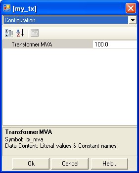
Module Parameters Dialog |
|
|
||
|
|
||
|
|
||
|
Module Definition Circuit Canvas |
||
Figure 2-7 – Passing an Input Parameter to the Module Canvas
Whatever value is now entered into the module parameter tx_mva, will be imported into the module canvas, where it is defined as a data signal, and may be collected by any component with a compatible input parameter. Let’s have a look at some bits of the Fortran files generated when this project is built. First of all, the Main.f file will contain four subroutines: DSDyn, DSOut, DSDyn_Begin and DSOut_Begin. Each of these subroutines will contain a call to the corresponding subroutine declared in the file my_tx.f. Notice that an argument containing the value of the module input parameter exists as part of the subroutine call statement. This allows for different values to be passed in to the subroutine, depending on the module instance.
|
! -1:[my_tx] CALL my_txDyn(100.0)
|
Listing 2-4 – my_tx Module Call in Main.f Subroutines
The my_tx.f file will also contain four subroutines, representing the my_tx module. These are: my_txDyn, my_txOut, my_txDyn_Begin and my_txOut_Begin. Making up the body of these subroutines will be the extracted code from the components defining the module (in this case mainly the 3 Phase 2 Winding Transformer).
Now let’s consider what happens if a second instance of the my_tx module is created, and its input parameter given the value of 200.0 MVA. Following rebuild, the project will still have only two Fortran files associated with it. This is because there are still only two module definitions. However, the second instance of the my_tx module will result in an additional call to the my_tx subroutines in the Main.f file.
|
! -1:[my_tx] CALL my_txDyn(100.0) ! -1:[my_tx] CALL my_txDyn(200.0)
|
Listing 2-5 – my_tx Module Call in Main.f Subroutines (Two Instances of Child Module)
Note this time how the module parameter values differ between calls. This is because of the change in value for the second instance of the my_tx module.
The my_tx.f file remains unchanged.
In system dynamics terms, each module instance is represented by a call to its corresponding subroutine (one call within each dynamics section). The calls will always be located within the subroutine body of its parent module. In most cases, the Main module is the top-most parent. However other modules can act as parents if the project hierarchy is more than two levels deep.
In many cases, it is possible that certain component input parameters may be dependent on the instance of the module in which the component resides. That is to say that one or more parameters may differ depending on the calling point of the module subroutine in the system dynamics. This is where the BEGIN subroutine and its inherent storage arrays come into play.
EXAMPLE 2-3:
Consider a user-defined module, which contains the simple control circuit illustrated below.
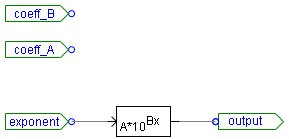
Figure 2-8 – User-Defined Module Circuit Canvas
The canvas contains a single master library component called Exponential Functions, which can be adjusted to represent exponential functions of base 10 or base e (in this case it is set to base 10). The component will also accept values for a base coefficient A, as well as an exponential coefficient B. These two component input parameters are both of type Constant and are described as Coefficient of Base and Coefficient of Exponent respectively.
There are two port connections defined for the module: One is an input connection called exponent, which represents the value of the exponent itself; and output, which is the result of base 10 taken to the exponential value. There are also two module input parameters called Base Coefficient and Exponential Coefficient with Symbol name coeff_A and coeff_B, which import the parameter values onto the canvas.
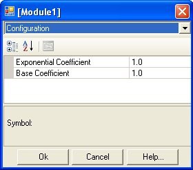
Figure 2-9 – User-Defined Module Input Parameters
The above described system will allow the module itself to be instantiated many times, with each instance able to possess unique values for both the exponent and the two coefficients. For example, let us create a second instance of this module and place them both in a circuit on the main canvas as shown below.
Figure 2-10 – Two Instances of a User-Defined Module on the Main Canvas
The Fortran segment in the Exponential Functions component definition contains a #BEGIN directive block, which specifies that the script within the block is to be inserted into the BEGIN section of the system dynamics. Since this directive is located in the Fortran segment, PSCAD will decide in which subsection of BEGIN to insert the code (i.e. in this case it will be the Module1Dyn_Begin subroutine). Let’s look at the Module1.f file following a build.
|
! SUBROUTINE Module1Dyn_Begin(coeff_B_, coeff_A_) ! ! . . . ! ! Subroutine Parameters REAL coeff_B_, coeff_A_ ! Control Signals REAL coeff_B, coeff_A ! ! . . . ! coeff_B = coeff_B_ coeff_A = coeff_A_ ! ! . . . ! ! -1:[exp] Exponential Functions RTCF(NRTCF) = coeff_A RTCF(NRTCF+1) = coeff_B NRTCF = NRTCF + 2 ! RETURN END ! SUBROUTINE Module1Dyn(exponent_, output_, coeff_B_, coeff_A_) ! ! . . . ! ! Subroutine Parameters REAL exponent_, coeff_B_, coeff_A_ REAL output_ ! Control Signals REAL exponent, output, coeff_B, coeff_A ! ! . . . ! exponent = exponent_ coeff_B = coeff_B_ coeff_A = coeff_A_ ! ! . . . ! ! -1:[exp] Exponential Functions ! output = RTCF(NRTCF) * 10**(RTCF(NRTCF+1) * exponent) NRTCF = NRTCF + 2 ! ! . . . ! RETURN END
|
Listing 2-6 – Segments of the Module.f File
Within the Module1Dyn_Begin subroutine (i.e. the BEGIN section of the system dynamics), the input parameter values for each instance of the module are stored in the RTCF storage array and the corresponding NRTCF pointer is incremented. During runtime, these same storage locations are accessed within the DSDYN subroutine Module1Dyn.
EXAMPLE 2-4:
Consider the circuit described in Example 2-2. The 3 Phase 2 Winding Transformer component is runtime configurable because it comes complete with BEGIN section source. The DSDYN segment in its definition contains a #BEGIN directive block, which specifies that the script within the block is to be inserted into the BEGIN section of the system dynamics. Since this directive is located in the DSDYN segment, the script will be inserted specifically into DSDYN subsection of BEGIN (i.e. the my_txDyn_Begin subroutine).
|
#BEGIN #LOCAL REAL RVD1_1 #LOCAL REAL RVD1_2 #LOCAL REAL RVD1_3 #LOCAL REAL RVD1_4 #LOCAL REAL RVD1_5 #LOCAL REAL RVD1_6 #LOCAL INTEGER IVD1_1 RVD1_1 = ONE_3RD*$Tmva RVD1_2 = $V1~ #CASE YD1 {~*SQRT_1BY3} {~} RVD1_3 = $V2~ #CASE YD2 {~*SQRT_1BY3} {~} CALL E_TF2W_CFG($#[1],$Ideal,RVD1_1,$f,$Xl,$CuL,RVD1_2,RVD1_3,$Im1) CALL E_TF2W_CFG($#[2],$Ideal,RVD1_1,$f,$Xl,$CuL,RVD1_2,RVD1_3,$Im1) CALL E_TF2W_CFG($#[3],$Ideal,RVD1_1,$f,$Xl,$CuL,RVD1_2,RVD1_3,$Im1) IF ($NLL .LT. 0.001) THEN RVD1_5 = 0.0 RVD1_6 = 0.0 IVD1_1 = 0 ELSE RVD1_6 = $NLL RVD1_4 = 6.0/($Tmva*RVD1_6) RVD1_5 = RVD1_4*RVD1_2*RVD1_2 RVD1_6 = RVD1_4*RVD1_3*RVD1_3 IVD1_1 = 1 ENDIF CALL E_BRANCH_CFG($BR11,$SS,IVD1_1,0,0,RVD1_5,0.0,0.0) CALL E_BRANCH_CFG($BR12,$SS,IVD1_1,0,0,RVD1_5,0.0,0.0) CALL E_BRANCH_CFG($BR13,$SS,IVD1_1,0,0,RVD1_5,0.0,0.0) CALL E_BRANCH_CFG($BR21,$SS,IVD1_1,0,0,RVD1_6,0.0,0.0) CALL E_BRANCH_CFG($BR22,$SS,IVD1_1,0,0,RVD1_6,0.0,0.0) CALL E_BRANCH_CFG($BR23,$SS,IVD1_1,0,0,RVD1_6,0.0,0.0) CALL TSAT1_CFG($BRS1,$BRS2,$BRS3,$SS,RVD1_1, #IF SAT==1 +RVD1_2, #ELSE +RVD1_3, #ENDIF +$Xair,$Xknee,$f,$Tdc,$Im1,$Txk) #ENDBEGIN
|
Listing 2-7 – 3 Phase 2 Winding Transformer Component #BEGIN Directive Block
Now let’s look at the my_tx.f file following a build.
|
! SUBROUTINE my_txDyn_Begin(tx_mva_) ! ! . . . ! ! Subroutine Parameters REAL tx_mva_ ! Control Signals REAL tx_mva ! ! . . . ! ! -1:[xfmr-3p2w] 3 Phase 2 Winding Transformer 'T32' RVD1_1 = ONE_3RD*tx_mva RVD1_2 = 230.0*SQRT_1BY3 RVD1_3 = 230.0 CALL E_TF2W_CFG((IXFMR + 1),0,RVD1_1,60.0,0.1,0.0,RVD1_2,RVD1_3,0.& &4) CALL E_TF2W_CFG((IXFMR + 2),0,RVD1_1,60.0,0.1,0.0,RVD1_2,RVD1_3,0.& &4) CALL E_TF2W_CFG((IXFMR + 3),0,RVD1_1,60.0,0.1,0.0,RVD1_2,RVD1_3,0.& &4) IF (0.0 .LT. 0.001) THEN RVD1_5 = 0.0 RVD1_6 = 0.0 IVD1_1 = 0 ELSE RVD1_6 = 0.0 RVD1_4 = 6.0/(tx_mva*RVD1_6) RVD1_5 = RVD1_4*RVD1_2*RVD1_2 RVD1_6 = RVD1_4*RVD1_3*RVD1_3 IVD1_1 = 1 ENDIF CALL E_BRANCH_CFG( (IBRCH(1)+1),SS(1),IVD1_1,0,0,RVD1_5,0.0,0.0) CALL E_BRANCH_CFG( (IBRCH(1)+2),SS(1),IVD1_1,0,0,RVD1_5,0.0,0.0) CALL E_BRANCH_CFG( (IBRCH(1)+3),SS(1),IVD1_1,0,0,RVD1_5,0.0,0.0) CALL E_BRANCH_CFG( (IBRCH(1)+4),SS(1),IVD1_1,0,0,RVD1_6,0.0,0.0) CALL E_BRANCH_CFG( (IBRCH(1)+5),SS(1),IVD1_1,0,0,RVD1_6,0.0,0.0) CALL E_BRANCH_CFG( (IBRCH(1)+6),SS(1),IVD1_1,0,0,RVD1_6,0.0,0.0) CALL TSAT1_CFG( (IBRCH(1)+7), (IBRCH(1)+8), (IBRCH(1)+9),SS(1),RVD& &1_1,RVD1_2,0.2,1.25,60.0,1.0,0.4,0.1) ! RETURN END
|
Listing 2-8 – Segment of the my_tx.f File
Within the my_tx Dyn_Begin subroutine (i.e. the BEGIN section of the system dynamics), the entire contents of the #BEGIN directive block can be found. This chunk of code contains calls to subroutines internal to EMTDC, which perform variable initialization and storage so as to ensure that the 3 Phase 2 Winding Transformer component is indeed runtime configurable.