Ideal Transposition of Aerial Conductors
Practical Cable Cross-Bonding of Underground Cables
Many long AC transmission lines employ the concept of conductor transposition in order to minimize system imbalance. In a practical sense, this is achieved by periodically rotating the conductor positions in the circuit, so that each phase spends an equal distance in each position, between the sending and receiving end.
Figure 8-15: Practical Transposition Cycle of a 3-Phase Circuit
There are essentially two methods by which to model practically-connected, transposed lines in PSCAD (valid when using the Bergeron and either of the Frequency Dependent line models). The first method requires that each section of the total line to be represented as an individual line. The transpositions can be implemented in one of two ways for this case: The first is to physically transpose the circuit interconnections between the line sections on the PSCAD Canvas, as shown below:
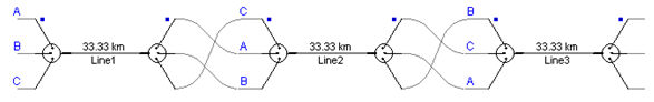
Figure 8-16: Practical Transposition of a 100 km Overhead Line in PSCAD
An alternative method is to alter the conductor XY coordinates within the properties editor of each line section. One benefit of this method is that phase A could remain conductor #1 throughout the length of the transmission line.
Practical transposition, like that described above, minimizes system imbalance caused by conductor positioning, but does not completely remove it. The system becomes more and more balanced as the number of transposition cycles increase (and hence the segment lengths decrease), from one end to the other. For studies where it is desirable for line to be completely balanced, the LCP provides an option called 'Ideal Transposition'.
Ideal transposition is a mathematical average of the unbalanced line. This is equivalent to visualizing an infinite number of transposition cycles, where the line segment length approaches zero. The result is a series impedance matrix Z and a shunt admittance matrix Y that are perfectly symmetrical and balanced. For example, if Zsc is the system impedance matrix, then Z'sc is it’s ideally transposed equivalent:
|
|
(8-44) |
Where,
|
|
(8-45) |
|
|
(8-46) |
The PSCAD Master Library supplies a few towers containing multiple circuits, which include additional options for ideal line transposition. When using these components, users may opt to either transpose each circuit separately, or include all circuits in the transposition calculation. If the latter option is chosen, then the transposition procedure is as described in the previous section. However, if the circuit transposition is performed on a circuit-by-circuit basis, then the procedure is slightly different. For example, it is required that a three-phase, double-circuit tower be separately ideally transposed. Then for the system series impedance,
|
|
(8-47) |
Where,
Z1, Z2, Z'1 and Z'2 are defined separately as given by Equation 8-42 and:
|
|
|
|
|
|
Practical transposition can also be performed on underground, single-core coaxial cables called 'Cross-Bonding'. This method is similar to that performed on overhead lines, but in this case the respective conducting layers are switched, while the core conductor remains untouched. Please note that Ideal transposition is not available for underground cables systems in the LCP.
Figure 8-17: Major Section of Cross-Bonded Sheaths for Three Single-Core Cables in PSCAD
Many practical underground cable systems employ the cross-bonding of sheath conductors in order to reduce circulating currents. The sheaths are transposed at regular intervals (similar to transposition of phases in the overhead lines in many ways). One way to represent a cross-bonded cable is by splitting the cable into small cable sections (as described above), where the sheaths between two cable sections are interchanged accordingly. However, in many practical situations, the number of cable sections may be very high (ex. A 25 km cross-bonded cable with 400 m cable sections needs 62 unique cable models in the simulation project). The 62 cable models require higher computational effort and memory compared with a single 25 km cable model and also much smaller time step significantly reducing the simulation speed.
Ideal cross-bonding is an alternative way to include cross-bonding to the existing cable line model (see reference [31]). The cable sheath can be assumed as cross-bonded through the entire length of the line (similar to the ideal transposition option in overhead lines). This is a good approximation for situations where there are many cross-bonded sections. This method gives sufficient accuracy for studies including switching transient studies and fault analysis. An additional advantage of this method is that simulation speed is much higher than the conventional approach.
Figures 8-18a and 8-18b show the simulation results for a three cable system. A step voltage is applied to the conductor of the first cable and receiving-end of the same cable is short-circuited at t = 0.1 s. All other conductors (including sheaths) are connected to ground through 1 W resistance. The figures compare the current through the conductor of the first cable and the induced voltage on the conductor of the second cable for three cases, ideal cross-bonded cable system, actual cross-bonded with 9 cross-bonded major sections and a non cross-bonded system. There is a significant mismatch between the cross-bonded and non cross-bonded cable results. Simulation results for ideal cross-bonded system are in a close agreement with cross-bonded case. If there are large number of cross-bonded sections (typical in many practical applications), the ideal cross-bonding is a good approximate for the actual cross-bonded system.
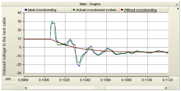
Figure 8-18a: Comparing Induced Voltage in Ideal, Actual and Non Cross-Bonded Systems
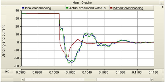
Figure 8-18b: Comparing Sending-End Current in Ideal, Actual and Non Cross-Bonded Systems