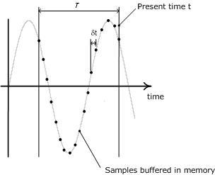
This subroutine provides an RMS quantity for a 1-phase, repeating input waveform such as a sinusoid, by interpolated sampling. A given number of samples per cycle of fundamental frequency (NSAMI) are continuously buffered in memory, thus providing a 'moving snapshot' of the input signal. The snapshot boundaries are defined by the present time t and the period T of the fundamental frequency (FREQ). The sample period dt is of course defined by both the NSAMI and FREQ inputs.

Overview of the DGTL_RMS Meter
The main benefit of this meter over the equivalent [RMS3] Analog RMS Meter (1-Phase) is that it provides a very smooth output signal, which may be necessary when used as input in some control circuits. However, due to its 'moving snapshot' or 'buffered' approach, the DGTL_RMS meter does not respond as quickly as the RMS3 function to changes in input signal state.
Sampling the Input Data
This subroutine first considers the input number of samples per cycle NSAMI and ensures that the number is appropriate, given the input frequency FREQ and the chosen simulation time step DELT. If the product of these three values (i.e. NSAMI x FREQ x DELT) is greater than or equal to 1.0, then the number of samples per cycle is adjusted internally according to:
![]()
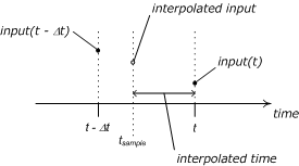
This alters the number of samples requested (called NSAM), if the time step and/or frequency is too large to accommodate the given number of samples per cycle. If a sample time falls between time steps (which is normally the case), the subroutine will adjust the input value through linear interpolation (based on the input from both the present and the previous time step), and use the interpolated input value in the calculation of the output.

Output Calculation
The output is refreshed whenever a sample time is encountered, as described above, based on the input quantities stored in the input buffer. The output RMS signal is given by:

|
Subroutine Author(s): |
O. Nayak |
Nayak Corporation, 2003 |
SUBROUTINE DGTL_RMS(NSAMI,FREQ,INPUT,SCALE,INIT,OUTPUT)
Inputs:
|
Argument |
Type |
Dimension |
Description |
|
|
|
|
|
|
NSAMI |
INTEGER |
1 |
The number of samples to be taken per cycle of fundamental frequency input FREQ. This input affects the number of storage locations used by this subroutine (see below). |
|
FREQ |
REAL |
1 |
The fundamental frequency of the INPUT signal [Hz] |
|
INPUT |
REAL |
1 |
The input signal on which to calculate the RMS value. |
|
SCALE |
REAL |
1 |
A constant to scale the output value (ex. a per-unitizing base). This value is multiplied directly to the OUTPUT signal internally. |
|
INIT |
REAL |
1 |
Initial output value (optional). The subroutine populates the entire buffer with this value at TIMEZERO. |
Outputs:
|
Argument |
Type |
Dimension |
Description |
|
|
|
|
|
|
OUTPUT |
REAL |
1 |
Output RMS signal. If SCALE = 1.0, then this output will be in the same unit as the INPUT signal |
This function requires the following storage allocations per call (see #STORAGE Script Directive and STORx Arrays for more details):
#STORAGE INTEGER:2 REAL:<?> *See Note Below*
|
Address |
Description |
|
|
|
|
NSTORI + 0 |
The present sample number |
|
NSTORI + 1 |
The adjusted number of samples per cycle (normally equal to NSAMI). See the Description above for more details. |
|
NSTORF + 0 |
Sample period = 1 / FREQ*NSAMI. Minimum is the simulation time step DELT [s]. |
|
NSTORF + 1 |
The time at which to take the next sample [s] |
|
NSTORF + 2 |
Input from last time step |
|
NSTORF + 3 |
Output from last time step |
|
NSTORF + 4...4+NSAMI |
Buffered input array. Note that the quantities stored here are the squares of the inputs at each sample point. |
NOTE: The total number of REAL storage locations used is: REAL = 4 + <value of NSAMI>. It may actually be less than this, but this depends on what the subroutine decides is a valid number of samples, taking into account the input FREQ and the simulation time step DELT. Using the value of NSAMI is a safe choice. You may monitor the actual number of samples by accessing NSTORI + ? as indicated above.