Selection of Switching Resistance
Switching and non-linear elements are those that change state during a simulation, according to certain conditions. These devices can range from simple switching elements, such as power electronic devices, (i.e. thyristors, diodes, etc.), breakers and faults, to more complex non-linear elements that can have many states, such as the arrestor.
In addition to those with many states, non-linear devices can also be modeled with an additional compensating current source that can be programmed to represent any non-linearity.
There are several different methods for representing a simple switching element in time domain simulation programs [5]. The most accurate approach is to represent them as ideal. That is, possessing both a zero resistance in the ON state and an infinite resistance in the OFF state.
Although this approach is very accurate and the resulting equations easier to solve, the drawback is that many possible states are created, which must each be represented by different system equations.
EXAMPLE 3-2:
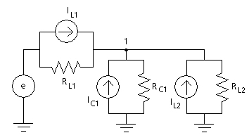
Consider the network of Figure 3-3 and let the resistance R12 represent a simple switch. If R12 were considered ideal, then two different networks could result, depending on the state of the switch. This is illustrated in Figure 3-4:
Figure 3-4 (a) - ON State of an Ideal Switch
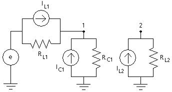
Figure 3-4 (b) - OFF State of an Ideal Switch
Now imagine for instance, a network containing many switches (as in a 48-pulse Graetz bridge STATCOM), a great number of different possible network configurations would result if ideal switching elements were used.
In EMTDC, simple switching devices are represented as a variable resistor, possessing an ON resistance and an OFF resistance. Although this type of representation involves an approximation of both the zero resistance (ON) and an infinite resistance (OFF) of an ideal switch, it is advantageous in that the same circuit structure can be maintained, and the electric network will not need to be split into multiple networks, as a result of each switching event.
In EMTDC, there are provisions to allow for zero resistances (see Ideal Branches). However, while the ideal branch algorithm is very reliable and gives the theoretical result, it does involve extra computations to avoid a division by zero when inverting the conductance matrix. Thus, by inserting a reasonable resistance typical of a closed switch, you can improve the simulation speed. A non-zero value larger than 0.0005 W should be used wherever possible.
Selection of the switching resistances is important: If the resistance is too small, its value may dominate the conductance matrix and the other diagonal elements could be overshadowed or lost. This will cause its effective conductance matrix inversion to be inaccurate.
NOTE: The default ON resistance value in PSCAD is 0.001 W. The threshold, under which the Ideal Branch algorithm will be invoked, is 0.0005 W.
These important factors should be kept in mind when choosing a switch resistance:
Circuit losses should not be significantly increased.
Circuit damping should not be reduced significantly: Due to the solution being in steps of discrete time intervals, numerical error may create less damping in the circuit than expected in reality. A small amount of additional resistance from a closed switch, if judiciously selected, may compensate the negative damping effect in the solution method.
There are two methods for representing non-linear elements in EMTDC: The Piecewise Linear, and the Compensating Current Source methods. Each method possesses its own pros and cons, and the selection of either is simply up to the user.
Although a non-linear device may possess a characteristic that is continuous, controlling the device as continuous is not recommended: Continually changing branch conductance can force a conductance matrix inversion every time step, resulting in a substantially longer run time in large networks.
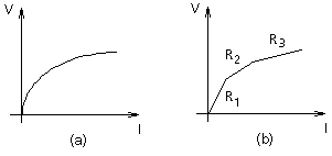
Figure 3-5 - (a) Continuous (b) Piecewise linear conductance properties
In order to minimize run time, a Piecewise Linear approximation method as illustrated in Figure 3-5 (a) and (b) is used. A piecewise linear curve will introduce several 'state ranges' into the non-linear characteristic, dramatically reducing the amount of matrix inversions per run, yet maintaining reasonable accuracy.
In EMTDC, non-linear devices, such as the Arrestor component, utilize the Piecewise Linear technique.
Another method to modeling a non-linear characteristic is through the use of a compensating current source. This technique is accomplished by adding an equivalent Norton current source in parallel with the device itself, thereby allowing for the addition or subtraction of extra current at the device branch nodes.
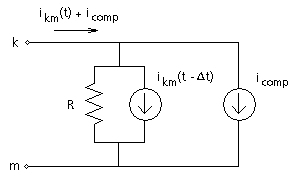
Figure 3-6 - Compensating Current Source Method
Care must be taken when using this method to model device non-linearities. More often than not, the compensating source will be based on values computed in the previous time step, thereby behaving as an open circuit to voltages in the present time step. This can create de-stabilization problems in the simulation [5]. To circumvent this problem, the compensating current source should be used in conjunction with a correction source and terminating impedance. See Machine Interface to EMTDC and/or [5] for more details on this concept.
In PSCAD, the compensating current source method is used to model core saturation in the Classical Transformer models.