My First Automation Script

Launch Enerplot

The following script is the starting point for all Enerplot scripting. It establishes a connection to the Enerplot application. If Enerplot is not running, the Enerplot application will be started.

#!/usr/bin/env python3
import mhi.enerplot

# Launch or Connect to the Enerplot application
enerplot = mhi.enerplot.application()

When the script is run, Enerplot will launch, if it is not already open. If Enerplot is already running, or if this script is run from inside Enerplot, no effect will be visible.

Load a Workspace

Add the following lines to the script:

# Load the Enerplot_Examples workspace
enerplot.load_workspace("Enerplot_Examples", enerplot.examples)

This requests Enerplot load the “Enerplot_Examples.epwx” workspace.

The second argument is an optional directory to load the workspace from. Instead of hard-coding the path C:\Users\Public\Documets\Enerplot\1.0.0\Examples, we ask Enerplot for its “Examples” directory, to simplify locating the desired workspace.

When this script is run, whatever workspace is loaded by default is replaced with the “Enerplot_Examples” workspaces.

Unload a Book

The “notes” book is unnecessary documentation; we can remove it from the workspace. Add the following lines to the end of the script:

# Get rid of the `notes` book.
notes = enerplot.book("notes")
notes.unload()

When the script is run, after the workspace is loaded, the “notes” book will be removed.

Create a Sheet

Inside of “book1”, we will create a new sheet for our experimentation. Add the following lines to the end of the script:

# Add a new sheet to "book1"
book1 = enerplot.book("book1")
sheet2 = book1.new_sheet("Sheet2", "Created by Python script")
sheet2.focus()

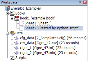
When the script is run, the “Sheet2” tab is selected (by the sheet2.focus() command) so that the newly created empty sheet is automatically displayed.

The newly created sheet can also be seen in the Workspace tree when the “book1” node is expanded.

Add a Graph Frame

On this newly created sheet, we will create a graph frame, set the title of the frame, as well as change the x-axis label from “x” to “Time”, with the following additional lines of code:

# Add a graph frame, with title and x-axis label
frame = sheet2.graph_frame(1, 1, 40, 36, title="Cigre Rectifier", xtitle="Time")

The 1, 1, positions the graph frame 1 grid unit from the left edge and top edge of the sheet; the 40, 36, sets the graph frame’s width to be 40 grid units wide and 36 grid units high.

It could have been done in individual steps with:

# Add a graph frame
frame = sheet2.graph_frame()
frame.position(1, 1)                                        # Move from the default position
frame.size(40, 36)                                          # Change the size from the default
frame.properties(title="Cigre Rectifier", xtitle="Time")    # Change title & x-axis label

Add Curves to Graph

To add curves to the graph, we first need to access the channels in a data file. Begin by obtaining a handle to the datafile, and select 3 channels from within it:

# Add Rectifier AC voltages to the graph frame's top graph
cigre = enerplot.datafile("Cigre_47.csv")
ph_a = cigre["Rectifier\\AC Voltage:1"]
ph_b = cigre["Rectifier\\AC Voltage:2"]
ph_c = cigre["Rectifier\\AC Voltage:3"]

Once handles to the 3 channels have been acquired, we can obtain a handle to the top (currently the only) graph in the graph frame, and add the curves to that graph. Finally, we can zoom in on the beginning of the graph, to show the start-up detail.

top = frame.panel(0)
top.properties(title="Phase Voltages (kV)")
top.add_curves(ph_a, ph_b, ph_c)
top.zoom(xmax=0.15, ymax=1.0, ymin=-0.2)

Additional Graphs

Since we’ll be adding more information to the graph frame, to keep things organized, we’ll create a second graph inside the graph frame for the additional curve.

# Add second graph to graph frame
bottom = frame.add_overlay_graph()
bottom.properties(title="Zero Sequence Voltage (V)")

Creating New Data

The real power of scripting Enerplot from Python comes from using Python to perform virtually any operation the user can describe programmatically. In this case, we’ll start with a relatively simple operation: computing the Zero Sequence of the 3-phase AC Rectifier Voltage.

Earlier, we retrieved handles to 3 channels: ph_a, ph_b and ph_c. Each channel represents a series of values over a domain, time in this case. We can pull that data (the series of values) from Enerplot into Python by access the channels’ .data members. For instance, the first few samples from each of those channels:

>>> for i in range(5):
            print(ph_a.data[i], ph_b.data[i], ph_c.data[i])

1.9361584377011e-22 1.9361584377011e-22 1.9361584377011e-22
7.2525547995022e-06 -0.00012775595458015 0.00012050339978074
6.3961421264228e-05 -0.00058302843340511 0.0005190670121476
0.00022705364312596 -0.0014130327742065 0.0011859791312948
0.00055983463703418 -0.0027041771168113 0.0021443424820356

Adding corresponding sample values together will produce the zero sequence voltage. Multiplying the resulting sum by 1000 will convert the result to volts. This can be done for every point in the time domain with one Python statement, using the zip() function and list comprehension:

v_zero = [ (va+vb+vc)*1000 for va,vb,vc in zip(ph_a.data, ph_b.data, ph_c.data) ]

Once the desired signal has been created, it must be passed back to Enerplot for display in graphs. Since data can only be displayed from a channel in a datafile, we must create a new channel in the datafile for the newly created signal before it can be added to a graph. Add the following to the script:

# Create Zero Sequence channel
v_zero = [ (va+vb+vc)*1000 for va,vb,vc in zip(ph_a.data, ph_b.data, ph_c.data) ]
zero_seq = cigre.set_channel(v_zero, "Zero Sequence", "Script Output")
bottom.add_curves(zero_seq)

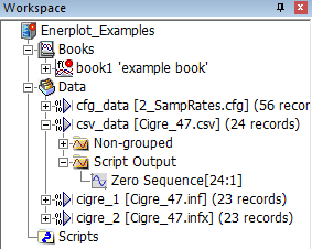
If you expand the “Cigre_47.csv” data node, you can see a new “Script Output” group, with the newly created “Zero Sequence” channel.

Note

It is important to recognize that, like the “Record Wizard”, this data has not been stored in the “Cigre_47.csv” datafile. Unlike channels created by the Record Wizard, this data will not be regenerated when the workspace is reloaded. It can only be generated by re-running the script.