As discussed in Chapter 3, transient simulation of an electric network, over a certain period of time, is accomplished by solving the network equations at a series of discrete intervals (time steps) over that period. EMTDC is a fixed time step transient simulation program and therefore, the time step is chosen at the beginning of the simulation, and remains constant thereafter.
Due to the fixed nature of the time step, network events such as a fault or thyristor switching, can occur only on these discrete instants of time (if not corrected). This means that if a switching event occurs directly after a time step interval, then the actual event will not be represented until the following time step.
This phenomenon can introduce inaccuracies and undesired switching delays. In many situations, such as a breaker trip event, a delay of one time step (say about 50 ms) is of hardly any consequence. However, in power electronic circuit simulation, such a delay can produce very inaccurate results (i.e. 50 ms at 60 Hz is approximately 1 electrical degree). One way to reduce this delay is to reduce the time step. However, this will also increase the computation time proportionately, and still may not give good enough results.
Another method is to use a variable time step solution, where if a switching event is detected; the program will sub-divide the time step into smaller intervals. However, this does not circumvent the problem of spurious voltage and current spikes, due to current and voltage differentials when switching inductive and capacitive circuits.
EMTDC uses an interpolation algorithm to find the exact instant of the event if it occurs between time steps. This is much faster and more accurate than reducing the time step and interpolation allows EMTDC to accurately simulate any switching event, while still allowing the use of a larger time step.
Here is how it works:
Each switching device adds its criteria to a polling list when called by the DSDYN subroutine. The main program then solves for the voltages and currents at the end of the time step, while storing the switching device condition at the beginning of the time step. These devices may specify a switching instant by time directly, or by voltage or current crossing levels.
The main program determines the switching device, whose criteria for switching has been met first, and then interpolates all voltages and currents in this subsystem to that instant in time. The branch is then switched, requiring a re-triagularization of the conductance matrix.
EMTDC then solves for all history terms, increments forward by one time step past the interpolated point, and solves for the node voltages. All devices are polled to see if more interpolated switching is required before the end of the original time step.
If no further switching is required, one final interpolation is executed to return the solution to the original time step sequence.
These steps are illustrated in Figure 4-1:
Figure 4-1 - Illustration of Interpolation Algorithm
NOTE: If there is more switching in this particular time step, then steps 1 to 3 are repeated.
EXAMPLE 4-1:
Referring to Figure 4-2, let us consider a diode that is conducting, but should turn off when the current reaches zero. When the diode subroutine is called from DSDYN at time step 1, the current is still positive, so no switching occurs.
If interpolation is not available (or turned off in EMTDC), a solution at time step 2 would be generated. The diode subroutine would then recognize that its current is negative, and subsequently switch itself off for time step 3 - thus allowing a negative current to flow through the device.
Figure 4-2 - Non-Interpolated Diode Current
In EMTDC (with interpolation turned on), when the diode subroutine is called from DSDYN at time = 1, it still of course would not switch the device off because the current is positive. However, because this is a switch-able branch, it would be part of a list indicating to the main program that if the current through this branch should go through zero, it should switch the branch off before the end of the time step.
The main program would generate a solution at time = 2 (as it did above), but would then check its list for interpolation requirements. Since the new diode current is negative at time = 2, the main program would calculate when the current actually crossed zero. It would interpolate all voltages and currents to this time (say time = 1.2), and then switch the diode off.
Assuming that there is no further switching in this time step, the main program would appropriately calculate the voltages at time = 1.2 and 2.2 (1.2 + Dt), and then interpolate the voltage back to time = 2 to bring the simulation back on track with integral time steps.
Figure 4-3 - Interpolated Diode Current
NOTE: DSDYN and DSOUT are still only called at times, 1, 2 and 3, yet the diode is still turned off at 1.2, so therefore no negative current is observed.
The main program would then call DSOUT so that the voltages and currents at time = 2 can be output. It would then call DSDYN at time = 2, and continue the normal solution to time = 3.
There is one additional complication to the above procedure: A chatter removal flag (see Chatter Detection and Removal) is automatically set any time a switch occurs. The flag is cleared as soon as an uninterrupted half time step interpolation is achieved. In the example above, this means that an additional interpolation would be performed to 1.7 (half way between 1.2 and 2.2), a solution at 2.7, and then the final interpolation would return the solution to 2.0 as before.
To prevent an excessive number of switches in one time step, the solution will always proceed forward by at least 0.01% of the time step. In addition, any two (or more) devices, which require switching within 0.01% of each other, will be switched at the same instant.
As an example of the application of interpolation, a simple HVDC system, where the differences in measured alpha (at the rectifier) for a constant alpha order is illustrated in Figures 4-4 (a) and (b), with a 50 ms simulation time step. While the interpolated firing produces less than 0.001° fluctuation, the non-interpolated firing results in about 1° fluctuation. Such large fluctuations (of one or more degrees) in firing will introduce non-characteristic harmonics and will prevent fine adjustments in firing angles. In these two examples, EMTDC automatically interpolates the thyristor turn off to the zero crossing (negative) of the thyristor current.
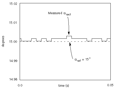
Figure 4-4 (a) - Example of Interpolation Effect: Interpolated
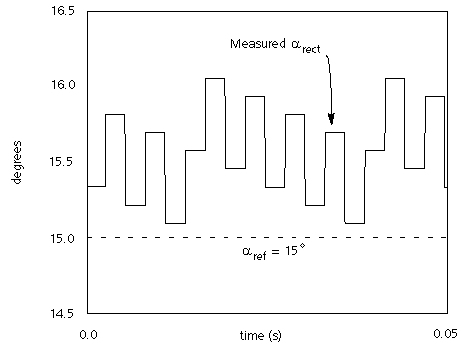
Figure 4-4 (b) - Example of Interpolation Effect: Non-interpolated
Example applications where interpolation is advantageous:
Circuits with a large number of fast switching devices
Circuits with Surge Arresters in conjunction with power electronic devices
HVDC systems with synchronous machines which are prone to Sub-Synchronous Resonance
Analysis of AC/DC systems using small signal perturbation technique where fine control of firing angle is essential.
Force commutated converters using GTO's and back diodes
PWM circuits and STATCOM systems
Synthesizing open loop transfer functions of complex circuits with power electronic devices
For more details on interpolation, please see [6], [7] and [8].