DC Correction

Issues with Fitting Transfer Matrices at Low Frequency

DC Correction by Changing the Functional Form

DC Correction by Adding a Pole/Residue

High voltage direct current (or HVDC) transmission over long distances has seen ever increasing application all over the world.  Simulation models for such systems are continually being pushed to the limit; requiring accuracy over a wide range of frequencies, including 0 Hz or DC.  Up until recently, transmission properties at DC were based on a best approximation, where the error could vary greatly depending on the system being simulated.

As discussed in previous sections, the use of modern phase domain modeling techniques, coupled with parameter estimation using Vector Fitting, has greatly improved the accuracy of time-domain models for transmission lines and cables.  Although the frequency-dependent models simulate the frequency range from a default of 0.5 Hz to about 1 MHz, it has been difficult to achieve a good fit in the proximity of 0 Hz (DC).  When dealing with HVDC lines and cables, it is very important to accurately reproduce the response at DC, as this is the nominal frequency of the line.  It can be shown that forcibly trying to fit the characteristics at these extremely low frequencies requires high order fitting and sometimes leads to inaccurate results.

A feature exists in the Line Constant Program that modifies the form of the rational function, approximated in the curve fitting procedure, when using the Frequency-Dependent (Phase) model only.  The rational function approximations, for both the propagation and the characteristic admittance matrices, can be fitted more accurately without having to substantially increase the number of poles.  In fact, with this approach the DC response is exact!  This feature is called DC Correction.

DC Correction allows for two possible variants of the functional form.  In the first approach, the admittance and propagation transfer functions are reformulated so that the DC response is factored out as an additive constant, which can then be directly selected.  In the other approach, the transfer function is first fitted over the entire frequency range, which typically results in some fitting error at precisely DC.  A low frequency first order pole is then added to the resultant fitted function in order to realize the exact response at DC, without significantly affecting the remainder of the frequency response.

Also see Chapter Reference [27] for more detailed reading.

Issues with Fitting Transfer Matrices at Low Frequency

At very low frequencies, the equations for A and Yc reduce to,

Where,

The square root term in Equations 8-80 and 8-81 does not permit a rational function approximation with a low order; and thus a higher order rational function may be needed for the fitting if very low frequencies are considered.

Consider for example, a simple three single-core coaxial cable configuration shown below:

Figure 8-24 – Simple Three Single-Core Cable Configuration

A typical frequency response of the Yc(1,1) element (i.e. the core admittance of cable 1) is shown in Figure 8-25, which also shows a plot of a rational function approximation obtained by limiting the lower fitting frequency bound to 1 Hz.

Figure 8-25 – Characteristic Admittance Response of a Simple Three Single-Core Cables

Notice that the fitting at frequencies below the lower bound is poor.  The response with a lower bound of 1 Hz, which is often selected by users when studying DC systems, can produce a significant steady-state error.  Reducing the lower bound to 0.1 Hz, reduces the error, but achieves this with a significant increase in the fitting order as discussed earlier.  Note that poor fitting at very low frequencies is a major source of error when modelling DC lines.

DC Correction by Changing the Functional Form

If Equations 8-71 and 8-79 are re-written in an equivalent form (Equations 8-82 and 8-83 respectively), it is readily seen that setting s = 0 results in a single term, which is the response at DC (i.e. the term ddc,theoretical).

By selecting ddc,theoretical to be precisely the known DC value, a perfect fit at DC is guaranteed.  This approach has been introduced in the Frequency-Dependent (Phase) model, as discussed in [27].  These modified equations can be re-expressed in a similar form to Equations 8-71 and 8-79, so as to make the formulation amenable to the vector fitting process.  Using a proper choice of variables, Equation 8-83 can be converted into a form as shown in Equation 8-84, which is suitable for vector fitting.

Where,

A minor issue with the above method is that although the DC error is eliminated, the resultant propagation function at very large frequencies deviates marginally from zero; which is contrary to the physical properties of typical propagation functions. Although the error introduced is trivial, the terms in Equation 8-84 can be slightly perturbed, using another least squares fitting, to taper the high frequency response to zero, without altering the correct DC value.

As seen in Figure 8-26, this approach results in an excellent fit over the entire frequency range, without any increase in the order of the fitted function.  The corresponding time domain results for a short circuit on the cable in Figure 8-24 is shown in Figure 8-27.  Over a 10 second interval, accurate reproduction of the response is shown when compared to a solution using numerical inverse Laplace transform methods.

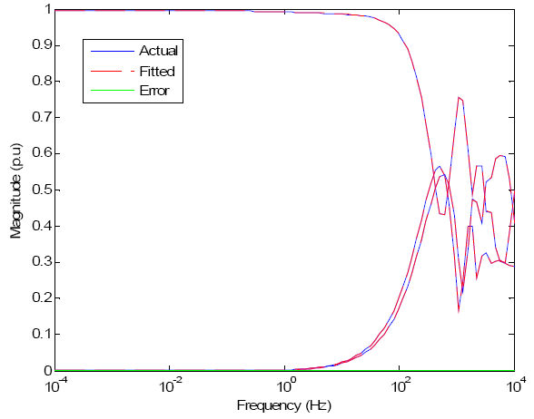
Figure 8-26 – Frequency Response Plots for the Elements of the First Column of the Propagation

Figure 8-27 – Time domain Results for a Short Circuit Condition

DC Correction by Adding a Pole/Residue

The known characteristics (i.e. elements of the admittance and propagation matrix) are first fitted with a rational polynomial, as is done conventionally for the Frequency-Dependent (Phase) model. First, a real pole with a suitable residue c0 is added to it, so that the modified function gives the exact value at DC. This modification increases the order of the rational function by one order of magnitude, and does not affect the high frequency asymptote.  Also, as the cut-off frequency of the additional term is smaller than the lower fitting bound, this correction is achieved with a very small error to the fitted part.

Figure 8-28 – Magnitude of A(1,1) Before and After the Addition of Pole/Residue

The choice of a0 (or k in above paragraph) is selected by another optimization process that minimizes the error between the actual frequency response, and that of fmod. As seen in Figure 8-28, the pole at frequency 2π x 0.5 Hz gives the most accurate response at frequencies approaching DC, as well as the closest fit over the entire low frequency range. The corresponding time domain simulations for the line current are shown in Figure 8-29, where the superior accuracy of the 2π x 0.5 Hz pole in the simulation is evident. In the above case, the original function was fitted with a lower frequency bound of 1 Hz, so as to limit the transfer functions to lower orders.

Figure 8-29 – Sending-End Current of First Conductor with Different Poles Selected