Frequency-Dependent Network Equivalent (FDNE) (2024)

This component is used to create a multi-port, frequency-dependent network equivalent from given characteristics, such as impedance (Z), admittance (Y) or scattering (S) parameters. This model first approximates the parameters with rational functions using the Vector Fitting technique. Once the parameters are expressed in rational form (pole/residue) or state-space form, an EMT-type, frequency-dependent network equivalent can be constructed, consisting of admittances and current sources.

In power systems, a Frequency-Dependent Network Equivalent (FDNE) model may typically be used to represent many system types, including wide-band, reduced-order network equivalents, high-frequency power transformers, or short transmission lines; all from frequency sweep measurements/computations. This component can be used to model high-frequency power electronic converters and filters as well.

NOTE: This component is a result of a collaborative effort between Manitoba Hydro International, Ltd. and SINTEF Energy Research. Specifically, the Y and S-parameter models (Admittance and Scattering parameters) were contributed by SINTEF.

Input Data

Input to this component is the frequency-dependent characteristics of the network to be represented by an equivalent, and is provided as a text file. The input data may be given in one of the following formats:

*Note: In the Interface to Harmonic Impedance Solution component, the Impedance Output Type parameter must first be set to Phase Impedances, prior to producing output.

Output Data

The component instance number and call number are used to create detailed output files (ex. fdne_<instance number>_<call number>.log) in the project temporary folder.

These output files are created in the project temporary folder when the Detailed Log File parameter is set to Create. It is advisable to check log files to make sure that the FDNE solution is accurate.

Passivity Enforcement

Time domain simulations can be sometimes unstable due to passivity violations [40]. A passivity enforcement algorithm is implemented to enforce stability for the frequency range defined in the passivity identification.

Power Injections

The FDNE component can be used to model a portion of a network (sub-network) using parameters, such as impedance or admittance (these parameters only represent a passive network). However, the sub-network may consist of active elements, such as voltage sources, etc. The effect of active elements can be modeled by defining power injections at the component terminals. This will give accurate power flow and terminal voltages. When the terminal conditions (voltage, angle, active and reactive power) or current injections are defined, the model automatically calculates the current injections.

Connection Port Assignments

Input Parameters

Name for Identification	Text		Optional text parameter for identification of the component.

Total Number of Ports	INTEGER	Literal	This is the total number of ports (or electrical connections) to the network equivalent component.

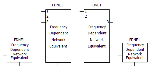
Number of Ports on One Side	Choice		This parameter may be used to configure port positions on the component graphic. For example, this may be useful to model a frequency-depended transformer with primary and secondary terminals on both sides. Enabled only if Graphics Display \| Expanded is selected.

Reference Port	Choice		Select Ground or External Connection. If External Connection is selected, the reference will be made available for external connection on the component graphic, via a connection port.

Detailed Log File	Choice		Select Create or Do Not Create.

View	Choice		Select Expanded or Compact. Compact mode is the general, multi-port connection (up to 100 nodes). Electrical Tap components may be used to connect to the external network. The expanded connections are limited to 10.

Input Data File	Text		Enter a the name of the input data file.

Path to Input File	Choice		Select Relative or Absolute. Select Relative if you are giving the input data file name as relative to the current working folder. Use absolute path if you are giving the data file name as an absolute path (ex. C:\temp\harm.out).

Data Format	Choice		Select From Harmonic Impedance Component, Impedance Parameters, Scattering Parameters, Admittance Parameters, Admittance as ABCD Parameters or Scattering as ABCD Parameters or Sequence Parameters. Select the type of input data to be used to calculate the network equivalent. See Input Data File Format for details.

Curve-Fitting Technique	Choice		Select from three available techniques to fit the frequency-domain data Fast Vector Fitting (FVF), Fast Relaxed Vector Fitting (FRVF) or Fast Modal Vector Fitting (FMVF). Fast Vector Fitting (FVF) is the original vector Fitting method [28]. Fast Relaxed Vector Fitting (FRVF) provides an improved pole relocation, hence increases the accuracy of the fitting [48]. Fast Modal Vector Fitting (FMVF) enforces accuracy of admittance and impedance parameters simultaneously [49]. It provides a major improvement in accuracy for cases with high ratios between the largest and smallest eigenvalues.

Type of Rational Function	Choice		Select Proper or Strictly Proper. Typically, the default setting Proper is fine for many characteristics. However, if you want to enforce the admittance to be zero at high frequencies, use Strictly Proper. If a Strictly Proper rational function is selected, the order of the numerator will be less than denominator order. On the other hand, if a Proper rational function is selected, the order of numerator and denominator will be equal. The main difference is that a proper approximation will never grow unbounded as the frequency approaches infinity, while a strictly proper approximation will approach zero as the frequency goes to infinity.

Maximum Fitting Error (%)	REAL	Literal	Enter the maximum error allowed for the curve fitting process [%]. The program will incrementally increase the order of the approximation to fit the data until this error criterion is met. However, the resulting number of poles is not allowed to exceed the specified Maximum Order of Fitting.

Starting Order of Fitting	INTEGER	Literal	Enter the staring order for fitting the transfer function (usually 1). By default, the selected curve-fitting technique starts the rational approximation from an order of 1 and increases the order until the fitting error is less than the user-specified value. In case some information regarding the system is known, one can start the fitting process from a higher order, saving computational time and resources.

Order Incrementation	INTEGER	Literal	This is the amount by which the order is increased in each step. Increasing this value can lead to a faster convergence.

Maximum Order of Fitting	INTEGER	Literal	Enter the maximum number of poles to be used for curve-fitting. The order of rational function on the Kth step will be: ORDER_ST+(K-1)*ORDER_INCR <= ORDER However, overfitting and passivity violations can happen if the order is increased excessively.

Type of Weighting	Choice		Select Common or Independent. If Common is selected, a united weighting factor is applied to all the matrix elements in a specific frequency. If Independent is selected, matrix elements are weighted independently.

Weighting Scheme	Choice		Select User-Defined or Strong Inverse or Weaker Inverse. If User-Defined is selected, enter the weighting factor applied at different frequency intervals (W1, W2 and W3). If Strong Inverse is selected, the frequency-domain response becomes weighted with the inverse of its magnitude ( 1 / \|f(s)\| ). This is useful when a frequency-domain response has both large and small values and the fitting error needs to be minimized over all the elements. If Weaker Inverse is selected, the square root of the inverse of the magnitude (1 / √(\|f(s)\| )) is applied as the weighting factor.

Steady State Frequency	REAL	Literal	Enter the system steady-state frequency (F0) [Hz]. This is only important, if you want to define different weighting functions between different bands of frequencies (see below).

Weighting Factor for Minimum to Steady Sate Frequency	REAL	Literal	Provide a weighting factor for the frequency range Fmin to F0. Note: The minimum frequency Fmin is the minimum frequency defined in the data file.

Weighting Factor for Steady State Frequency	REAL	Literal	Provide a weighting factor for the steady-state frequency F0.

Weighting Factor for Steady State to Maximum Frequency	REAL	Literal	Provide a weighting factor for the frequency range F0 to Fmax. Note: The maximum frequency Fmax is the maximum frequency defined in the data file.

Enforce Passivity?	Choice		Select No, Yes (Perturbation method) or Yes (Filter method). Select Yes (Perturbation method) to enforce stability of the time domain simulation by calling the perturbation-based, passivity enforcement algorithm. Select Yes (Filter method) to enforce stability by calling the filter-based, passivity enforcement algorithm).

Maximum Error (%)	REAL	Literal	Maximum percentage error after passivity enforcement.

Maximum Iterations	INTEGER	Literal	Maximum number of iterations for passivity enforcement algorithm.

Starting Frequency	REAL	Literal	Starting frequency for passivity violation identification [Hz].

End Frequency	REAL	Literal	End frequency for passivity violation identification [Hz].

Number of Samples	REAL	Literal	Number of samples used for passivity identification.

Frequency Scale	Choice		Select Log, Log and Linear or Linear for passivity identification.

Rest of the File Name	Description
fdne_<instance number>_<call number>.log	Log file
fdne_<instance number>_<call number>_Y_MAG.out	Magnitude of actual and fitted admittance
fdne_<instance number>_<call number>_Y_ANG.out	Angle of actual and fitted admittance

Enable Power Injections	Choice	Select No, Yes (Boundary Conditions) or Yes (Current Injections). Select Yes (boundary conditions) to enable power injections through terminal conditions of the FDNE. Select Yes (Current Injections) to enter current injections directly at the terminals.

Input Data File	Text	Name of the input data file. See Input Data File Format.

Path to Input File	Choice	Select Relative or Absolute. Select Relative if you are giving the input data file name as relative to the current working folder. Use Absolute path if you are giving the data file name as an absolute path (ex. C:\temp\pq.out).