
Frequency-Dependent Transfer Function (FDTF) 2
Original date created: June 12, 2017
This component is used to model a dynamic system using a state-space representation. The component allows modelling of a multi-port transfer function, and therefore can be used with any other continuous system modeling functions (CSMF) in order to implement a complex control system. The state-space model has the form:
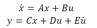
If the state-space model represents a multiple port system, then A, B, C and D are complex matrices.
Example 1: Initialization
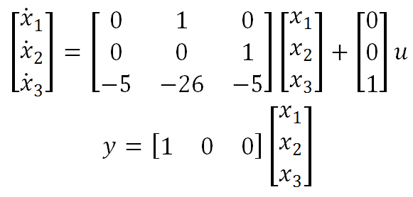
In this example, he dynamic response of the state-space model is compared for when the FDTF implementation has the parameter initialization set to Zero and input at time = 0. The following equations are used to represent the dynamic system.
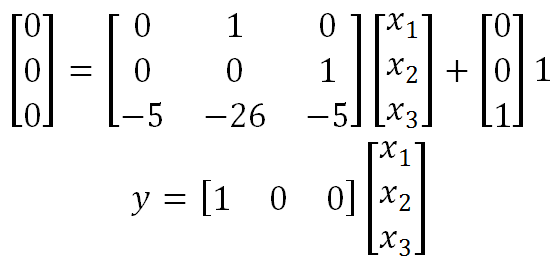
As illustrated by the simulation results, all the states are initialized to zero, and the output of the system is zero when the option Zero is selected in the FDTF component parameters. Otherwise, the FDTF calculates the state variables before starting the simulation, using the input values at time zero. In this case, the system input is equal to 1. Hence, the FDTF component solves the following system of equations:
Solving:
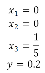
Therefore the output is 0.2, as can be verified in the simulation case.
Example 2: Canonical and Observable Forms
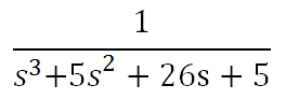
In this example, it is shown as to how two different FDTF models represent two identical, dynamic systems. Thus, it is verified that the state-space representation of a dynamic system is not unique. On the other hand, there is only one transfer function which can represent a dynamic system. For this example, we have chosen the following transfer function that has also been included in the simulation to compare the results.
The state-space representation that has been selected for the example are the controllable canonical, and the observable canonical forms.
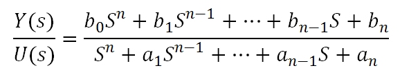
For a transfer function,
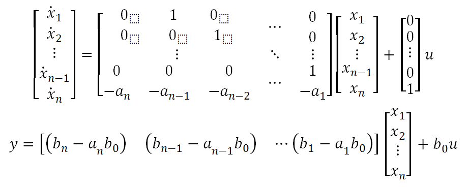
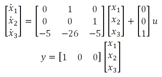
The controllable canonical form has the following representation:
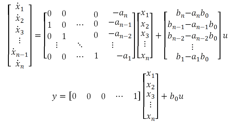
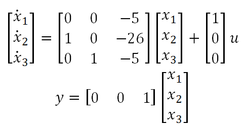
The equations for the observable canonical form are:
Therefore, the controllable canonical form of the transfer function is:
And the observable canonical form is:
It can be verified that the three output curves match perfectly in the simulation results.
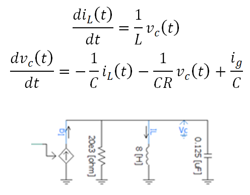
Example 3: RLC Circuit Representation
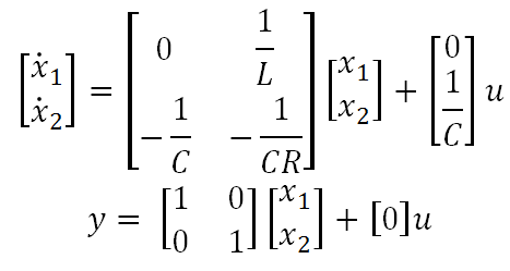
This example illustrates how to mimic the response of an RLC parallel circuit using the FDTF component. The circuit differential equations are:
Thus the equations can be written in matrix notation:
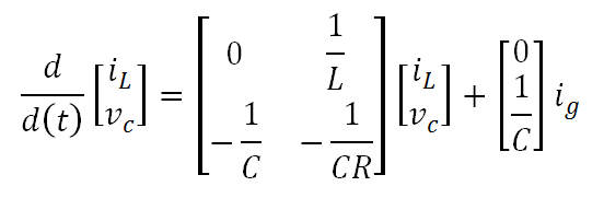
The state-space model can be written using the current in the inductor and the voltage in the capacitor as state variables. The FDTF can be used as a MIMO (Multiple Input Multiple Output) model, which allows adding both variables as outputs. Then formulation is:
The values chosen in this simulation example are R = 20 kΩ, C = 0.125 µF and L = 8 H. Hence the state-space matrices are:
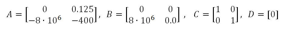
As can be verified in the simulation, both implementations produce the same results.