Users can generate custom records, based on existing records already loaded into the work environment, by using the record wizard.
The record wizard utilizes a text based math parser to calculate a new set of record data, based on the data from one or more existing records. Records may be added or subtracted from each other, for example. Or mathematical functions may be applied directly to a set of record data, such as a scale factor or other more complex operation.
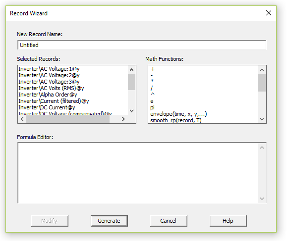
The record wizard environment is separated into the following areas:
Buttons:
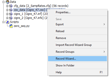
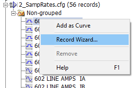
The record wizard may be accessed via either a dataset, Data branch or a record context menu:
|
|
Dataset Context Menu |
Record Context Menu |
Note that the selected record list that appears in the wizard, depends on the context in which it is invoked. If invoked from a dataset, all records in the set will appear and be available for use. If single or multiple records are selected when invoked, only the selected records will appear in the list.
To create a new record, you must first piece together a mathematical formula that describes the new record.
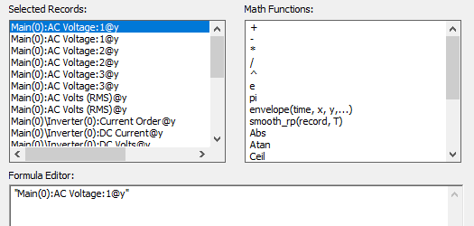
For example, say you want to add two voltages together, but first apply a scale factor of 1.3 to one of them. First double-click the first voltage record:
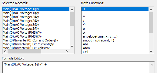
Next, double-click the + symbol:
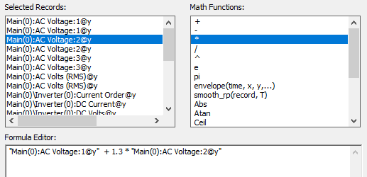
Now type 1.3 directly in the formula editor, double-click the * symbol, then double-click the second voltage record:
Press the Generate button.
A new record will be created and added to a folder (within that dataset) called Record Wizard Output. Simply add the new record to a graph, as you would any other record.
NOTE: The x-values of the new record are inherited from the record(s), on which it is based. Therefore, all records involved in the creation of this new record must all share the same x-axis.
The record comes complete with a list of basic mathematical functions, as described below:
Symbol |
Description |
Example |
^ |
Raised to the power of |
4 ^ 5 = 1024 |
* |
Multiply by |
3 * 6 = 18 |
/ |
Divide by |
9 / 2 = 4.5 |
+ |
Add |
1 + 1 = 2 |
- |
Subtract |
9 - 5 = 4 |
Min |
Minimum value |
min(10, 3) = 3 |
Max |
Maximum value |
max(1, 9, 2) = 9 |
Sin |
Sine |
sin(pi/2) = 1 |
Cos |
Cosine |
cos(pi) = -1 |
Tan |
Tangent |
tan(1) = 1.5574... |
Atan |
Arc tangent |
atan(0) = 0 |
Abs |
Absolute value |
abs(-8) = 8 |
Exp |
e to the power of |
exp(3) = 20.08... |
Log |
Natural log |
log(16) = 2.77... |
Ceil |
Round up |
ceil(6.2) = 7 |
Int |
Truncate to an integer |
int(6.8) = 6 |
Sqr |
Square root |
sqr(64) = 8 |
time |
A variable used to get record abscissa (x-axis data). |
time = 0.0, 0.001, ... |
e |
Exponent |
e = 2.7182818284590... |
pi |
Pi |
pi = 3.141592653589... |
In addition, there are a couple of preprogrammed functions as well:
Symbol |
Description |
Example |
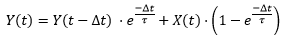
smooth_rp(record, T) |
This function simulates a lag or 'real pole' function. The time domain solution algorithm is based on the trapezoidal rule. The solution method for this function is as follows:
Where, Y(t) – Output signal X(t) – Input signal τ – Time constant (real) Δt – Time step interval And, Record – Used as the input signal T – Time constant, real value in seconds |
smooth_rp("Rectifier\DC Current@y", 0.05) |
Envelope (time, x1, y1, x2, y2, …) |
This function is essentially a piece-wise linear look-up table, where the x and y-coordinate points can be specified.
Where, time – Used as the input signal. Time variable is set as default. x1, y1, x2, y2, … - Used as x, y pairs of coordinates in the look-up table. Coordinates should be sorted by ascending x-values. There should be one or more pairs of coordinates in the envelope. |
envelope(time, 0.02, 0.5, 0.07, 0.8, 0.1, 1) |